java -cp MotifLab.jar motiflab.engine.MotifLab -p <protocol> [-s <sequences>] [optional arguments]

  -input <dataname> <value>  

  -sequences "<genome build>,<region>,<segment size>,<collection size>,<overlap>"  

A sequence in MotifLab represents a segment of a DNA strand spanning a specified number of bases. Usually, a sequence object will represent a "real sequence" where the location of the sequence segment and the genome build it originates from is known. For example, a sequence could span the segment from position 157,342,949 to position 157,343,321 on the reverse strand of chromosome 2 from the human genome build "hg19". Alternatively, a sequence object could represent an "artificial sequence" which is not tied to a specific location or genome build (or a "real sequence" whose actual location or genome build is simply not known). In either case, a sequence object in MotifLab is merely an "empty" template that contains very little information in itself. Specifically, even though it is referred to as a "sequence", it does not contain information about the actual DNA sequence found at the associated location. This information is contained in DNA Sequence Datasets, a type of Feature Datasets that can annotate sequence segments with additional information.

The required attributes of a Sequence object is:

• Chromosome
• Start coordinate
• End coordinate
• Strand orientation (default is "direct")

If the chromosome is not known (for instance for artificial sequences), it can be set to "?". In MotifLab, chromosomes always start at position 1, and both the start and end coordinates are inclusive (although certain data formats, like BED, might treat this differently).

A sequence can optionally be associated with a single gene and can then be annotated with the gene's name and the position of the transcription start site and end site.

• Gene name
• TSS
• TES

In MotifLab v2, sequences can also be annotated with Gene Ontology terms and other user-defined properties.

Creating Sequences

Sequences are normally created in MotifLab via the "Add Sequences" dialog which can be opened by selecting "Add Sequences" from the "Data" menu or by pressing the double-helix button in the tool bar. In protocol scripts, it is possible to create single (artificial) sequences with specified lengths or (real) sequences defined in BED or Location formats. Multiple sequences can be created with a single command by importing sequence definitions from a Location-, BED- or FASTA-file into the default sequence collection called "AllSequences". The Location-format supports all kinds of sequence metadata (including genome build and location of TSS/TES), but BED-files only contain information about the chromosomal location for each sequence and not its genome build. It is possible to update the genome build for each sequence afterwards, however, with the set[property] command. When importing sequences from FASTA files, the sequence metadata will be included if this information is present in the header of each sequence. If no metadata is present, MotifLab will just create artificial sequences based on the lengths of the sequences found in the FASTA file.
Note that even though the FASTA file contains the actual DNA sequences, only the metadata/length of the sequences will be used to create sequence objects. To include the actual DNA sequence you must also create an additional DNA Sequence Dataset based on the same FASTA file.
One final way to create new sequences is to extract subsegments from existing sequences with the split_sequences operation.

Modifying Sequences

Because so many other data objects depend on sequences and the locations represented by these objects, sequence objects are usually not allowed to be changed or even renamed after they have been created. Especially, new sequences cannot be created nor can existing sequences be extended after feature datasets have been added (since there would be no feature data for the new sequence segments). However, sequences can still be cropped and dropped.

In MotifLab v2, a few sequence properties – namely "genome build", "TSS", "TES", "orientation" and "gene name" – are allowed to be changed after creation. In addition, sequences can be annotated with gene ontology terms and other user-defined properties. The properties of a single sequence can be modified by right-clicking on the name label for a sequence in the Visualization panel (to the left of the tracks visualization) and then selecting "Display sequencename" from the context-menu to bring up a dialog window. Properties for single sequences or collections of sequences can also be updated with the set operation.

Using Sequences

Individual sequence objects are rarely used directly in MotifLab, but are rather used as templates for other feature datasets or are referenced to (by name only) as part of collections, partitions and maps. Only a few types of analyses currently make use of information stored directly in sequence objects, such as gene ontology term enrichment analyses.

Sequence objects are used in MotifLab to refer to specific sequence segments of a genome, but this data type does not contain any additional information about what is going on at these locations (apart from some metadata). Further location-specific annotations are kept in feature datasets which come in three different types:

• DNA Sequence Datasets hold the actual DNA sequence from the corresponding sequence segment (one base letter for each position)
• Numeric Datasets hold information that can be represented numerically along the sequence (one value for each base position)
• Region Datasets hold information about discrete sub-segments with specific properties within the sequence segment

In MotifLab's graphical user interface, all Feature Datasets are listed in the "Features" data panel which is usually located at the top of the left panel, and the feature data tracks themselves are shown for each sequence in the Visualization Panel. You can configure the visual appearance of feature tracks by right-clicking on a dataset in the "Features" panel (or selecting multiple by holding down the SHIFT or CONTROL keys) and then select options from the context menu or with keyboard short-cuts.

DNA Sequence Datasets (also called DNA tracks or DNA sequence tracks) are used to hold the DNA sequence for a sequence segment, represented with one base letter for each position within the sequence. Most often, objects of this type will hold the original DNA sequence from that location, but this does not have to be the case. The DNA sequence could instead be a slightly modified version of the original sequence, a scrambled version or even a fully artificially created sequence. The base letters would normally be either A, C, G or T, but all types of letters are allowed in the sequence. For instance could N's or X's be used to mask portions of a sequence. Base letters can be in either uppercase or lowercase, and the case may or may not be important depending on the context and the tools used to analyze the sequence. For example, lowercase letters can be used to indicate repetitive segments of a sequence that should be ignored by a motif discovery tool.

DNA sequences are always stored relative to the direct strand internally in MotifLab (independent of the annotated strand orientation of the sequence), but DNA sequences can be converted on-the-fly to display or manipulate the sequence relative to either strand when necessary.

Creating DNA Sequence Datasets

DNA Sequence Datasets are normally imported from predefined tracks or loaded from files (in FASTA or 2bit format), but they can also be artificially created based on a background distribution.

Modifying DNA Sequence Datasets

The main operation for modifying DNA Sequence Datasets is mask, which can replace base letters in certain positions with new letters or change the case of the letters. In addition, the plant operation can insert new binding motifs for transcription factors into an existing DNA sequence.
The GUI's draw tool allows users to manipulate the DNA sequence by drawing or typing directly into the visualized track.

Using DNA Sequence Datasets

DNA sequence tracks are used as input to motif discovery and motif scanning tools (and also module discovery/scanning) and similar operations or tools that search DNA sequences for specific patterns (such as the search and score operations). Background Models can be derived from DNA tracks, and base frequency statistics can also be derived with the statistic operation or the GC-content analysis. Sequence dependent characteristics of the DNA helix, such as e.g. stacking energy and propeller twist, can be derived from a DNA track with the physical operation and represented with numeric tracks. In MotifLab v2 it is possible to extract the corresponding amino acid sequence from the DNA sequence for all six reading frames.

DNA sequence tracks can also be referenced in conditions, as demonstrated in the last example below. Here, segments of a DNA sequence masked with X's are used to derive a new Region Dataset representing these masked portions. This is done by first creating a Numeric Dataset with value 1 for every position with an X and then converting this numeric track to a region track.

Numeric Datasets (also called numeric tracks) represent information with one numeric value for each position within a sequence segment. The type of information stored in numeric datasets could be, for instance, (per base) phylogenetic conservation levels, physical or statistical characteristics of the DNA sequence/double helix (e.g. helix twist and roll, or local GC-content), the distance from each sequence position to some target feature, per base quality scores (for sequence reads), number of ChIP-seq tag counts per position, and position-specific priors used to guide motif discovery, to list but a few examples.

Creating Numeric Datasets

Numeric annotation tracks (based on e.g. data from UCSC Genome Browser or other databases) can be imported from preconfigured tracks or loaded from files in various formats. Numeric tracks can also be derived from information in other types of tracks. For example, Priors Generators can be trained with machine learning methods to predict the location of certain features based on combined information from several different tracks. The output from a Priors Generator is a numeric track where each position reflects a prior probability (or likelihood) that the position could overlap with the target feature (for example a TF binding site).

Modifying Numeric Datasets

Existing numeric datasets can be modified with arithmetic operations (increase, decrease, multiply and divide) or assigned explicit values with the set operation. They can also be transformed with various mathematical functions (including square root, logarithm and random number), the values could be normalized to a new range or thresholded to create "binary valued" tracks. All of these operations work on a position-by-position basis, but the apply operation will transform tracks with sliding window functions which allow the new value in each position to be derived from values of several positions in a neighbourhood around each sequence position.
In addition, the GUI's draw tool allows users to manipulate numeric datasets by drawing directly into the visualized track.

Using Numeric Datasets

MotifLab is an expansion of an earlier program called PriorsEditor whose primary purpose was for creating numeric tracks that could be used as position-specific priors to guide the motif discovery process. In addition, apart from being merely descriptive and informative, numeric tracks can be used in conditions to limit operations to certain positions in the sequence or to regions with certain value distributions within their sites.

Region Datasets (also called region tracks) contain sets of regions which are discrete segments of the sequence with associated properties. Such regions could represent e.g. genes, exons, coding regions, DNase hypersensitive sites, ChIP-seq peak regions, CpG-islands, repeat regions, SNPs and transcription factor binding sites. Each region has a location within its parent sequence defined by a start and end position, and by extension also a length (which technically could be 0 but not negative) and genomic location (if the genomic location of the parent sequence is known). Other standard properties of regions include a type, a numeric score value and a strand orientation (which can be either "direct", "reverse" or "undetermined" and is relative to the genome not the parent sequence). Additional user-defined properties can be specified for regions as well, like for example the start and end coordinates for CDS subregions of genes or a "sequence" property for TFBS regions denoting the actual binding sequence at the particular site. These user-defined properties can either have boolean, numeric or textual values.

Regions in the same track may overlap with each other, and regions are also allowed to extend beyond the boundaries of their parent sequence (and could in theory also be located fully outside the sequence). The consequences of regions extending outside of a sequence may differ depending on the particular operation or analysis applied to region tracks.

Motif track
A motif track is a special kind of region dataset where the type properties of the regions refer to known motifs. Some operations, like motifDiscovery and motifScanning will always return motif tracks, and the motif track status is normally preserved when tracks are manipulated with other operations as well. When region datasets are imported from files or preconfigured tracks, the regions are checked to see if they could potentially correspond to motif sites by comparing the regions' names and lengths to currently defined motifs. If enough regions match with known motifs, the dataset will automatically be converted to a motif track. Region datasets can also be converted to motif tracks manually by right-clicking on a region dataset in the Features Panel and selecting "Convert to Motif Track" from the context menu, or with the following display setting command: $motifTrack(<trackname>)=true.
Motif tracks are listed with names in boldface in the Feature Panel in MotifLab's graphical user interface.

Module track
A module track is a special kind of region dataset where the type properties of the regions refer to known modules. Some operations, like moduleDiscovery and moduleScanning will always return module tracks, and the module track status is normally preserved when tracks are manipulated with other operations as well. When region datasets are imported from files or preconfigured tracks, the regions are checked to see if they could potentially correspond to module sites by comparing them to currently defined modules. If enough regions match with known modules, the dataset will automatically be converted to a module track. Region datasets can also be converted to module tracks manually by right-clicking on a region dataset in the Features Panel and selecting "Convert to Module Track" from the context menu, or with the following display setting command: $moduleTrack(<trackname>)=true.
Module tracks are listed with names in bold italics in the Feature Panel in MotifLab's graphical user interface.

Nested track
A nested track is a special kind of region dataset where the regions may contain nested child regions. For example, in a gene annotation track the top-level gene regions could contain nested regions corresponding to exons within each gene. The module track type described above is actually a kind of nested track where the nested regions correspond to individual motif sites within the module. The extract operation can be used to create new (un-nested) tracks based on only the top-level regions or the child regions of a nested track.
Nested tracks are listed with names in italics in the Feature Panel in MotifLab's graphical user interface.

Creating Region Datasets

Region annotation tracks (based on e.g. data from UCSC Genome Browser or other databases) can be imported from preconfigured tracks or loaded from files in various formats. Operations that search for particular patterns within DNA sequences (including motifDiscovery, motifScanning, moduleDiscovery, moduleScanning and search) will usually return the resulting matches as a region track, and regions can also be derived from numeric tracks with the convert operation. The extract operation can extract child regions from a nested track and also extract the start, end and center positions of regions.

Modifying Region Datasets

Operations targeting region tracks will either modify the properties of existing regions, remove regions from the track (filter and prune) or merge regions together. The start and end positions of regions cannot normally be manipulated directly (with e.g. set or arithmetic operations), but some operations like extend can change the size of regions and thereby also alter their location.

Most numerical operations that can be used to modify numeric tracks, numeric maps and numeric variables can also be applied to modify numeric properties of regions. Text properties can be altered with the set and replace operations. If the arithmetic operations (increase, decrease, multiply and divide) are applied to text properties of regions, they will function like set operations treating the properties as (comma-separated) lists of values. The increase and multiply operations will then function like set addition (union) whereas the decrease and divide operations will function like set subtraction. However, if arithmetic operations are applied to boolean region properties they function like the following boolean operators: increase = OR, multiply = AND, decrease = NOR, divide = NAND.

There are currently no operations that can add new regions to an existing region track, but the GUI's draw tool allows users to draw new regions directly into the visualized track, to delete existing regions and to modify a region's properties in a popup dialog.

Using Region Datasets

The primary purpose of MotifLab is to predict transcription factor binding sites and cis-regulatory modules within DNA sequences, and region datasets are used to represent such sites. In addition, apart from being merely descriptive and informative, region tracks can be used in conditions to limit operations to certain portions of the sequence. Several different analyses can be applied to region datasets to examine the coverage of the regions in a single dataset, to compare the overlap between two datasets, or to count the number of occurrences of each type of region in a dataset and compare this to another frequency distribution.

The Motif data type models the DNA binding recognition sequence of a particular transcription factor (or group of related factors).
Motif scanning tools can be used to predict potential binding sites for different transcription factors by searching DNA sequences for good matches to their corresponding motif models. MotifLab comes bundled with collections of experimentally determined binding motifs from several databases, including TRANSFAC and JASPAR. Novel motifs can also be predicted from sets of sequences with de novo motif discovery tools, or users can define new motifs directly by manually specifying a binding matrix, consensus sequence or explicit list of binding sequences.

Motif properties

The motif type is one of the richest data types in MotifLab in terms of the amount of different information it can contain.
A list of standard motif properties are described below. Except for "ID" and "matrix", all of these are optional.
In addition to these, motifs can also have extra user-defined properties.

Property	Description
ID	The ID or identifier of a motif is the same as the name of the motif data object. This is set when the data object is created and can not be changed later. The ID is usually in the form of a database specific identifier (e.g. M00037 or MA0004).
Short name	A concise name for the motif; usually an abbreviation of the name of the transcription factor such as "AP-1" or "CREB". Motifs from the TRANSFAC collection have short names on the form "X$yyy_nn" where X is a single letter code denoting a species group (V=vertebrates, I=insects, P=plants, N=nematodes, B=bacteria, F=fungi), yyy is a TF abbreviation and nn is either a quality code, consensus flag or incremental number (for discriminating between different motif models for the same factor).
Clean short name†	This is derived from the short name by stripping away the "X$" prefix and "_nn" suffix for TRANSFAC motifs so that only the TF abbreviation remains.
Long name	A longer name for the motif; usually the full name of the transcription factor such as "Activator Protein 1" or "cAMP-responsive element binding protein"
Names†	This is a list consisting of both the short name and the long name together with the names of all annotated binding factors
Presentation name†	This is a concatenation of the ID and the short name, e.g. "M00001-V$MyoD_01". This form is often used to refer to motifs in the GUI since the ID is usually not very informative by itself.
Size†	The size of the binding model (i.e. the length of the consensus sequence or number of rows in the binding matrix).
Matrix	A representation of the DNA binding sequence of the transcription factor in the form of a matrix model.
Consensus	A concise representation of the binding model in the form of an IUPAC consensus sequence, e.g. "sGGrnTTTCC". This property is usually derived from the binding matrix, but it is also possible to assign a new consensus sequence to the motif (in which case the the binding matrix will also be updated to correspond with the new consensus).
Matrix type†	This can be either count, frequency or weight depending on the format of the binding matrix
Support†	If the matrix is a count matrix this property returns the number of binding sequences that the model was based on (equal to the sum of one row in the matrix).
GC-content†	The fractional sum of G's and C's in the binding matrix. Reflects the factor's preference for binding to GC-rich sequences.
IC-content†	The information content of a matrix is a measure of its binding specificity which is again inversely related to the number of sequences the that motif will match. IC-content is usually correlated with motif size (longer motifs match fewer sequences) but more importantly with the amount of variation allowed by the binding motif (more degenerate motifs have lower IC and therefore match more sequences). The IC of a single position i within a motif is calculated with the formula:  2+∑b∈A,C,G,T  fb,i log2( fb,i ), where fb,i is the frequency of base b in position i, and the total IC of a motif is the sum over all positions. A position which only allows a specific base has the maximum IC of 2.0 and a position which does not show any preference towards a particular base has the minimum IC of 0. For a motif of length N the IC can thus range from 0 to 2*N (most specific).
Factors	Names of transcription factors associated with this motif. This could be a single factor or several related factors. It is also possible to include different aliases and synonyms for the same factor.
Classification	A class tag consisting of up to four numbers separated by dots, e.g. "3.5.1.2", where the first number identifies the superclass, the second number the class, the third number the family and the fourth number the subfamily of the transcription factor according to the classification hierarchy introduced by the TRANSFAC database.
Class name†	The corresponding name of the class tag. E.g. the class "3.5.1.2" has the name "Myb-like factors".
Description	A general description of the motif and its associated transcription factor(s) in free-text.
GO	A set of gene ontology terms that describe the transcription factor
Organisms	A list of species on which the motif model is based (or a list of species for which the motif model could potentially be relevant).
Expression	A list of tissue or cell-types where this transcription factor is known to be active
Alternatives	A list of other known motifs that cover the same transcription factor and are thus equivalent to this motif (but not necessarily 100% identical). The TRANSFAC and JASPAR motif collections that come bundled with MotifLab are annotated with known alternatives both within and between the collections.
Interactions	A list of other motifs that are known to interact with this motif (or rather, their TFs are known to interact). This information can be used to automatically create Module Collections from known interactions. It is also used by the "Interactions Viewer" tool to highlight binding sites for interacting factors in the vicinity of a selected target binding site. Of the motif collections that come bundled with MotifLab, only TRANSFAC is annotated with this kind of information.
Quality	A numeric quality measure ranging from 1 (best) to 6 that reflects the experimental reliability of the protein-DNA or miRNA-RNA interactions whose binding sites form the basis for this motif model. Functionally confirmed transcription factor or miRNA binding site Binding of pure protein or miRNA (purified or recombinant) Immunologically characterized binding activity of a cellular extract Binding activity characterized via a known binding sequence Binding of uncharacterized extract protein to a bona fide element No quality assigned
Part	Describes the portion of the binding recognition sequence required for protein binding and activation that is actually covered by this motif model. Full: This motif covers the full recognition sequence Halfsite: This motif only covers a small part of the full sequence required for binding and activation, for example half of a dimeric binding sequence. Dimer or Oligomer: This motif represents a concatenation of two or more binding sequences. Note that this information is not always reliable in the motif collections that come bundled with MotifLab.

^† These properties are derived from other properties and can not be altered directly.

Matrix model

The main way the binding motif is modelled in MotifLab is with a position-specific scoring matrix (PSSM), sometimes also called a position count matrix (PCM), position frequency matrix (PFM) or position weight matrix (PWM) depending on its format. This matrix is in the form of an N×4 table where each column represents one of the four DNA bases and each of the rows represent one position in the binding motif.

A simple count matrix can be created from a set of binding site sequences (aligned and of equal length) by going through each sequence position in turn, counting the number of times each base letter occurs in that position across all the sites and entering this number into the matrix at the corresponding row and column. For example, a matrix derived from the four 6bp binding sequences "CACGTG,CAGGTG,CACGTG,CACGTT" would look like this:

A	C	G	T
0	4	0	0
4	0	0	0
0	3	1	0
0	0	4	0
0	0	0	4
0	0	3	1

If a matrix is based on a large number of binding sites, the magnitude of the value for a particular base in row i relative to the other bases should approximate well the transcription factor's relative preference towards that base in that position of the binding recognition sequence.

A count matrix can be converted into a frequency matrix by dividing the value of each cell with the total sum of the row so that the combined frequencies of the four bases sum to 1.0 for each position. Such a frequency matrix can be further transformed into a weight matrix by replacing each cell value with the log-ratio log( f_i,b / p_b ), where f_i,b is the frequency of base b in position i and p_b is the background probability of observing that base in entire genome. A value of 0 for a base b at position i in a weight matrix thus means that the transcription factor shows no particular preference for that base in that position of the recognition sequence (taking the background distribution into account). A positive value reflects a higher preference for that base relative to the other bases and a negative value reflects a lower preference for that base.

When MotifLab imports motifs from a file, the matrix models will be kept in their original formats, but MotifLab also tries to detect what kind of format this is so that the matrix can be dynamically converted into other formats if necessary.
The rules for determining the format based on the matrix values are:

• If the matrix only contains positive integer numbers it is considered to be a count matrix
• If the matrix contains negative numbers it is considered to be a log-transformed weight matrix
• If all the values are between 0 and 1.0 and each row sums to 1.0 it is considered to be a frequency matrix
• If none of the above rules apply the matrix is considered to be an unnormalized frequency matrix

When converting a weight matrix into a frequency matrix, MotifLab will always assume a uniform background distribution ( p_b=0.25 for all bases).

Consensus model

A secondary way to represent the binding model of a motif is with a consensus string. This is a string of base symbols, one for each position in the binding motif, denoting either single DNA bases or degenerate bases that represent groups of two or more DNA bases with a single symbol.
The notation follows the standard suggested by IUPAC:

Symbol	Represents	Name	Complement
A	A	Adenine	T
C	C	Cytosine	G
G	G	Guanine	C
T	T	Thymine	A
R	A or G	Purine	Y
Y	C or T	Pyrimidine	R
M	A or C	Amino	K
K	G or T	Ketone	M
W	A or T	Weak	W
S	G or C	Strong	S
B	C, G or T	Not A	V
D	A, G or T	Not C	H
H	A, C or T	Not G	D
V	A, C or G	Not T	B
N	any base	Any	N

If a motif already has a matrix model, the correponding consensus string will be derived from that matrix in accordance with the rules outlined in the section below. If the motif has a consensus string but not a matrix model, a matrix will be constructed based on the consensus string.

Deriving an IUPAC consensus string from a matrix

1. A single base letter (A,C,G,T) is used if the frequency of that base is at least 50% and also at least twice the frequency of any other base
2. A double-degenerate letter (m,r,w,s,y,k) is used if the combined frequencies of two bases are at least 75%.
3. A triple-degenerate letter (b,d,h,v) is used if one of the bases has a frequency of zero.
4. If none of the previous rules apply, the wildcard letter 'n' will be used.

Deriving a matrix from an IUPAC consensus string

Creating motifs

Motifs are usually generated by motif discovery methods or loaded from pre-defined collections. However, it is also possible to define new motifs manually. In the GUI, select "Add New ⇒ Motif" from the "Data" menu or press the plus-button in the Motifs Panel and select "Motif" from the drop-down menu. This will bring up the Motif dialog. The dialog contains multiple tabs where you can enter values for various motif properties. The only required property is the binding motif itself, which can be specified either as a matrix model or a consensus sequence. Consensus sequences can be entered in IUPAC notation (see above) or as a list of individual binding sequences (separated by any non-letter character). The matrix model will then be created automatically from the consensus sequence. Note that if you create new motifs that are not part of collections, you must select to display "Motifs" from the drop-down menu in the Motifs Panel in order to see the motifs listed in the panel.

In a protocol you can create new motifs with the new operation as shown below. The argument should be a semicolon-separated list of "property:value" pairs. Semicolons within property values can be escaped with backslash. If property values are lists the entries should be separated with commas.

The only required property is the binding motif itself which can be specified either as an IUPAC consensus sequence ("CONSENSUS" property) or as a matrix model (by setting the properties "A", "C", "G" and "T"). Other standard properties include: SHORTNAME, LONGNAME, CLASS, ORGANISMS, PART, ALTERNATIVES, PARTNERS, QUALITY, FACTORS, EXPRESSION, DESCRIPTION and GO-TERMS (these names must be uppercase). All other specified properties are regarded as being non-standard, user-defined properties.

Examples

Motif manipulation

MotifLab v2 introduced several functions to derive new motifs based on existing motifs using the extract operation, including functions to reverse complement a motif, trim bases off the ends or even extend the motif with additional bases. These functions can be applied to both single motifs and collections (the syntax is almost identical in the two cases, except that the names of the single motif functions usually contain the word "motif" somewhere). When transforming a single motif in this way, the result must always be assigned to a new explicitly named motif object. However, when the operation is applied to a collection, the original motifs will be replaced with the new transformed motifs unless you specify a "name suffix" that can be used to derive sensible names for all the new motifs.

The following examples demonstrate all of the motif manipulation functions as applied to a full collection.
Remember to add the ";name_suffix=X" option after the extract function if you want to create new motifs rather than transforming the current.

Motif tracks

A motif track is a special type of region track where the regions correspond to motif sites. In these tracks the type property of each region site corresponds with the name of a motif. Motif tracks include meta-data properties that specifically tag them as such, and they can be recognized in the Features Panel by having names displayed in boldface font. Also, if you point the mouse at a motif track in this panel, the appearing tooltip will describe the dataset as being a "[Region Dataset, Motif track]".

Some operations, like motifDiscovery and motifScanning will always return motif tracks, and if you import a region track from any source, MotifLab will first check if it could potentially be a motif track and mark it as such if at least half of the first ten regions correspond to known motifs. You can also try to manually convert a regular region track into a motif track by right-clicking on a track in the Features Panel and selecting "Convert to Motif Track" from the context-menu.

A motif region or motif site is a region within a motif track that represents the location of a transcription factor binding site by having a type property that corresponds to the name of a known Motif model.


Motif tracks are given special treatment by the GUI's track visualizer, both with respect to how the motif regions themselves are drawn and also how their tooltips are rendered when you point the mouse at a motif region.

Motif match logos
When the track height and zoom level of the sequence in the sequence window allows it, motif regions will be drawn with motif match logos overlayed on top of the regions. These logos illustrate both the model of the motif itself and how well the model matches the DNA sequence at this particular location. They are inspired by the "Sequence logo" concept introduced by Schneider and Stephens ("Sequence logos: a new way to display consensus sequences", Nucleic Acids Research, Oct 1990, 18(20):6097-6100). The logo is created from the matrix model representation of the motif. For each motif position, the letters for the four bases are first drawn on top of each other. They will be sorted according to their frequency in the model, with the most frequent base on top. Each base letter is also scaled according to its frequency, so if e.g. the frequency of base "G" is 0.46, then the height of the letter G will take up 46% of the stack height, originally. Next, the whole stack of four base letters is scaled once again according to information content, so positions with higher information content (i.e. those whose frequency distribution is more skewed towards a single nucleotide) will have a higher stack. On the other hand, positions that have an almost uniform distribution between the four bases will have a very short height. In addition, the matching base at each position will be colored according to its base's preferred color, whereas the other bases will be drawn in a gray color. Consider as an example the motif region for "M00184 - MyoD" that the mouse cursor is pointing at in the image above. In the last position of this site, the motif model has an almost equal preference for the bases C and T, with C slightly preferred over T (since the most frequent base according to the model - here C - is drawn on top). However, the DNA sequence contains a "T" in this position rather than the most preferred base "C", as indicated by the fact that the T is colored red in the logo while the C is gray. The "colorfulness" of the match logo thus gives an indication of how well a motif model actually matches the DNA sequence at that location. The more tall letters drawn in vibrant colors the logo contains, the better the match between the motif and the sequence. Logos with lots of gray, on the other hand, indicate worse matches. It should be noted that the motif logo colors are not based on the match between the motif logo and the DNA track here seen above the motif track. The DNA sequence used when comparing the motif model to the sequence is taken from a property of the region itself, named "sequence" (this property can be inspected by double-clicking on a region). This "sequence" property is usually set automatically in each region when motif tracks are created based on DNA tracks (using motif discovery or motif scanning tools). Regions that lack this "sequence" property will not be drawn with overlayed motif match logos at all.


The visualization of motif sites and their tooltips will differ somewhat depending on whether the motif track is visualized in contracted mode or expanded mode, and the differences between these two modes are described below. You can switch between these modes by selecting a region track in the Features Panel and pressing the X or E keys, or by right-clicking on a track and selecting the mode from the context menu.

Expanded Mode
In expanded mode (shown in the image above), overlapping motif sites will be drawn beneath each other so that every region is clearly separated from the other regions and distinctly visible in the track.

• The "visualize score" option has no effect in this mode. All motif sites are drawn with the same height.
• If the "visualize strand (orientation)" option is enabled, the boxes of motif sites will be drawn with protrusions indicating their orientation (but only in zoom levels 1000% and above)

The tooptip for motif regions in expanded mode will include the following information (from top to bottom. See also example in figure above):

• The position that the mouse currently points to within the sequence followed by the name of the track (in boldface)
• The name (identifier) of the motif that the mouse is pointing at followed by the "long name" of this motif
• The third line contains additional information about this particular motif site:
  • The sequence span (length) of the region (in bp)
  • The orientation of the motif site
  • The score of the motif site
• The fourth line again shows the motif match logo where the base that the mouse is pointing to in the motif is highlighted with a pink rectangle. In front of the motif logo is a pair of nested boxes, where the outer box is white and the inner box has the color associated with the motif.

Contracted Mode
In contracted mode, all the regions are visualized on the same line and overlapping regions will thus be drawn on top of each other.

• When the "visualize score" option is enabled, the height of the regions will be scaled according to their scores.
• If the "visualize strand (orientation)" option is enabled, the track will be divided into two vertical halves by a middle line. Boxes drawn above this middle line indicate regions that have the same orientation as the orientation that the underlying sequence is currently visualized in. Regions that have the opposite orientation will be drawn with boxes below the middle line. Regions with undetermined orientation are drawn both above and below the line.

The tooltip shown when pointing at a position containing one or more regions will contain the position of the mouse pointer followed by the name of the track (in boldface). This information is then followed by one line for each region that overlaps with this position. Each line starts with a pair of nested boxes, where the outer box is white and the inner box has the color associated with the motif for that region. These boxes are followed by the match logo for the motif site where the position that the mouse currently points at is highlighted with a pink rectangle in the motif logo. If more than one region overlaps at this position, the logos for the different overlapping regions are aligned. The logos are followed by the name (identifier) of the motif, the motif's "long name", the region orientation, region size (in bp) and finally the region score.

The Module data type (also called composite motif or cis-regulatory module (CRM)) is used to model clusters of binding motifs that occur in relative proximity to each other and bind multiple TFs that cooperate in regulating one or more genes. The definition of a module can be loose (e.g. motifs A, B and C should all occur within a span of N bp) or very strict (e.g. the motifs A, B and C should occur in order with motif B located between 20 to 23 bp after motif A followed by motif C between 35 to 40 bp after motif B; in addition motif B should occur in reverse orientation relative to A and C).

Modules can either be defined manually, they can be discovered "de novo" from sequence data (either DNA tracks or motif tracks) by module discovery programs, or they can be derived based on interaction partner annotations in motifs. Once a collection of modules has been defined, the moduleScanning operation can be employed to search for instances of these modules in either motif tracks or DNA tracks (depending on the particular module scanning program used). Both the moduleDiscovery and moduleScanning operations will return module tracks, which are a special kind of region track where the type property of the regions correspond to module names. The regions of a module track are nested regions where the top-level regions correspond to the full module segment and the child regions correspond to the component motifs of the module.

Module definition

The definition of a module consists of two parts:

• A set of component motifs (sometimes also called module motifs or meta motifs)
• A set of constraints (optional)

Component motifs
A module represents a group of individual binding motifs which are referred to as the component motifs of the module. For example, in a module consisting of binding motifs for the interacting transcription factors SP1, NF-Y and SRF, the component motifs will of course be SP1, NF-Y and SRF. However, in MotifLab these component motifs do not correspond directly to the motif data type. Rather, component motifs represent an intermediate level of "meta-motifs" that are basically sets of equivalent binding motifs for the same TF. The reason for this is that a single TFs can be associated with multiple motif models (for example, the Heat Shock Factor has 12 different motif models in TRANSFAC Public alone!). So, if factor A is represented by N motifs and factor B has M motifs, one can simply define a single module for factors A and B rather than having to define N×M individual modules covering every possible combination of motifs for these two factors.

The figure on the right shows a module as it is displayed in the Motifs Panel. The structure of the module is visualized in a three-level hierarchy. The top-level is the module itself, named MOD0001 The second level is made up of 3 component motifs, named respectively SP1, NFY and SRF, and the third level lists the basic motif models associated with each of the component motifs (three models for SP1 and SRF and four models for NFY). Note that the colors used for the component motifs need not correspond to the colors for the individual motif models at the level below. Even thought the definition of the module allows its component motifs to be represented by multiple motif models, a specific module region (the occurrence of module site within a region track) will only have one motif model corresponding to each component motif site. For example, the module MOD0001 could be made up from TFBS corresponding to the motifs M00008 (SP1), M00209 (NF-Y) and M00152 (SRF) at one module site, but be made up of TFBS sites for M00255 (SP1), M00185 (NF-Y) and M00152 (SRF) in a different location. Since it is common for different motifs representing the same TF to have overlapping sites in a motif track, it would also be natural for the same module to have multiple overlapping sites representing different combinations of the underlying motif models. For example, if the MOD0001:SP1-NFY-SRF module existed at a particular location in the sequence and all of the underlying motif models matched their respective TF sites (3 models for SP1 and SRF and 4 for NF-Y), a straight-forward module scanning method could potentially predict 3x4x3=36 overlapping module sites for the same MOD0001 module at this location to cover all possible motif combinations. Note that it is also technically permissible for a module site to lack some of the component motifs.

Module constraints
In addition to the component motifs, the module can also be fitted with optional constraints. These constraints can either be global (applying to the module as a whole) or local (applying to a single component motif or the space between two component motifs).

Global constraints:
• Max span: The maximum width of the whole module. All the component motifs of the module must be located within a sequence window of this size
• Ordered: In an ordered module, the component motifs must appear in a specified order, whereas in an unordered module they can appear in any order. If the module is ordered, additional constraints can be placed on the distances between pairs of component motifs

Local constraints:
• Motif orientation: It can be specified that a component motif must have a certain orientation (direct or reverse) relative to other component motifs. Note that since this is relative, at least two motifs must have this constraint in order for this to make sense
• Distance between motifs: In an ordered module, it is possible to place constraints on the distance between two consecutive motifs. This could be a minimum distance, a maximum distance or both. Distances can also be negative (i.e. allowing overlap)

Module properties

A list of standard module properties are described below. In addition to these, modules can also have extra user-defined properties.

Property	Description
ID	The ID or identifier of a module is the same as the name of the module data object. This is set when the data object is created and can not be changed later. The ID is usually in the form of an incremental identifier (e.g. MOD1043), but it could also be a more descriptive name (as long as it adheres to the naming rules for data objects)
Component motifs	The "meta-motifs" (motif equivalence sets) that represent binding motifs for each individual binding factor in the module
Cardinality	The number of component motifs in the module (this is a derived property).
Max length	Also called "max width" or "max span". An optional global constraint specifying the maximum number of sequence bases that the module is allowed to span
Ordered	An optional global constraint specifying whether or not the component motifs must appear in a specific order within the DNA sequence
GO	A set of gene ontology terms that describe the module

Creating a module in the GUI

You can create a new module by selecting "Add New ⇒ Module" from the "Data" menu or alternatively pressing the "+" button in the Motifs Panel and selecting "Module" from the drop-down menu. Note that the modules you create will only be displayed in the Motifs Panel if the drop-down box above the panel is set to "Modules". Or if the modules are part of collections or partitions you can also see them by selecting these two options.

1) Specifying the component motifs
In the Module dialog, press the "Add motif" button to add a new component motif to the module. New motifs will be added to the end (right-hand side) of the module. By default, the module will be ordered, which is indicated with angular connector lines between the component motifs. If you uncheck the "Motifs must appear in order" box, the module will be unordered and the connector lines will not be displayed. It is currently not possible to rearrange the order of the component motifs within a module. You can remove a component motif by selecting it and pressing the "remove button". To select a component motif, simply point at the motif box (or above or below it) so that the box border changes to a red color, and then click. The selected portion of the module will be highlighted with a blue background, and all the settings that apply to this component of the module will be enabled in the dialog (such as name, select motifs, color and orientation).


Newly added component motifs will be given generic names on the form "MotifN", and the name will be flanked by stars in the motif box to indicate that the motif has not been associated with any actual motif models yet (e.g.  * Motif1 * ). You can change the name of a component motif in the "Name" text field of the dialog and also change the color by clicking the "Color" button.


To associate a component motif with actual motif models, either select a component motif and press the "Select motifs" button or double-click on the component motif in the visualization. This will bring up a motif browser where you can select which motifs models to use. Once a component motif has been assigned at least one model, the stars flanking the name in the motif box will disappear. You can hover the mouse over a motif box to see which motif models have been selected for that component. Note that all component motifs must have been assigned at least one basic motif, or else you will not be able to press the "OK" button to close the dialog and create the module.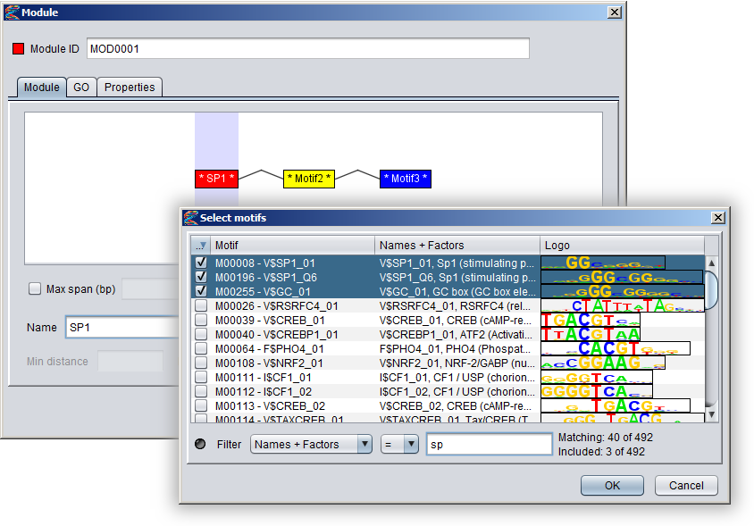


2) Setting distance constraints
You can specify a global max length for the module by checking the "Max span (bp)" box and then setting a number in the adjecent field. This constraint is taken to mean that all the component motifs of the module should be located within a sequence window of this size.

If the module is ordered you can also specify distance constraints between adjecent pairs of component motifs. To specify such a constraint, simply point to a connector line between motif boxes (the line should turn red), and click to select it. The selected connector should then be highlighted with a blue background, and the settings that apply to this connector will be enabled in the dialog. When you enter numbers into the min distance and max distance fields, these values will appear in brackets above the connector line. It is possible to leave one of the limits blank (either min or max) to say the the distance should be unconstrained in that direction. This will be marked with an asterisk in the brackets, as can be seen for the connector between the NFY and SRF motifs in the figure below. If both limits are left blank, the constraint will be removed.


3) Setting orientation constraints
It is possible to declare that the component motifs should occur in specific orientations relative to each other. To set an orientation constraint on a component motif, first select it in the visualization and then click on one of the colored arrow buttons underneath the "Add motif" button. If you select the "Direct orientation" button, a green right arrow will also be displayed above the component motif box in the visualization (see motif SP1 in the figure below), and if you select the "Reverse orientation" a red left arrow will be displayed above the motif box (motif SRF in the figure). If you select the yellow "any orientation" bidirectional arrow, the orientation constraint will be removed from the motif and no arrows will be displayed above the motif box (motif NFY in the figure).

Note that a direct orientation constraint does not imply that the motif has to be located on the direct strand (and likewise for reverse orientation). It simply means that the underlying motif model must match the DNA sequence in its default (not reverse) orientation, but this could potentially occur on either strand of the DNA sequence. Since orientation constraints are relative, they only make sense if at least two of the component motifs have such constraints.

Creating a module in a protocol

A new module can be created in a protocol script with the following general syntax:
The arguments are specified as a semicolon-separated list of property definitions, where the name of the property is case-sensitive. The first property argument must be CARDINALITY and its value must match the number of MOTIF arguments. The standard property arguments are described in the table below. Properties that are not in this table are considered to be user-defined properties and must be specified as "propertyname:value" pairs.

Property	Description
CARDINALITY	This defines the number of component motifs in the module on the format: CARDINALITY:<n> This must be the first argument!
MOTIF	Defines a component motif of the module on the format: MOTIF(<name>)[(<orientation>]{<list of motifs>} The "MOTIF" prefix is followed directly by a name for the component motif in parentheses. This is then followed by the orientation of the component motif in brackets. The orientation can either be "+" (direct orientation), "-" (reverse orientation) or "." (for unordered motifs). Finally, the basic motifs that make up this component motif is listed (comma-separated) within a pair of curly braces. For example, a direct-oriented component motif for the SRF transcription factor based on the three TRANSFAC models M00215, M00152 and M00186 can be defined as: MOTIF(SRF)[+]{M00215,M00152,M00186} Note that the "MOTIF" argument can be repeated several times, and the number of times it is used must match the CARDINALITY of the module.
ORDERED	Specifies that the component motifs of the module should be ordered. The order is based on the "MOTIF" arguments.
UNORDERED	Specifies that the component motifs of the module should be unordered. This is the default unless ORDERED is specified.
MAXLENGTH	Defines an optional maximum span for the module on the format: MAXLENGTH:<number of bases>
DISTANCE	Defines a distance constraint between two (consecutive) component motifs on the format: DISTANCE:(<motif1>,<motif2>,<min distance>,<max distance>) This only makes sense if the module is ORDERED. The minimum distance can be negative to allow overlapping motifs. If you only want to constrain one of the limits in the range (either min or max) you can set the other limit to UNLIMITED or *. This argument can be repeated several times to define distance constraints between different pairs of motifs. For example, if you want the distance between the two component motifs "SRF" and "NFY" to be at least 5bp, you can specify the constraint: DISTANCE(SRF,NFY,5,*)
GO-TERMS	Defines a set of GO-terms to be associated with the module on the format: GO-TERMS:<comma-separated list of terms> The GO terms are numbers that can optionally be prefixed by "GO:" (case-insensitive). The numbers do not have to be padded with zeros. The strings "GO:000290" and "290" will thus refer to the same term.

Module tracks

A module track is a special type of region track where the regions correspond to module sites. In these tracks the type property of each region site corresponds with the name of a module. Module tracks include meta-data properties that specifically tag them as such, and they can be recognized in the Features Panel by having names stylized in both bold and italics. Also, if you point the mouse at a module track in this panel, the appearing tooltip will describe the dataset as being a "[Region Dataset, Module track]".

Some operations, like moduleDiscovery and moduleScanning will always return module tracks, and if you import a region track from any source, MotifLab will first check if it could potentially be a module track and mark it as such if at least half of the first ten regions correspond to known modules. You can also try to manually convert a regular region track into a module track by right-clicking on a track in the Features Panel and selecting "Convert to Module Track" from the context-menu.

A module region or module site is a region within a module track that represents the location of a cis-regulatory module by having a type property that corresponds to the name of a known Module model. A module region is most often also a nested region where the child regions correspond to the individual TF binding sites that make up the module. These nested regions would then be motif regions whose type properties correspond to names of known Motif models. For example, in the figure below, a module model named MOD0001 is composed of two component motifs – HSF and TATA – with 9 and 6 associated motif models respectively. The particular module site corresponding to this module shown at the top of the track on the right would have the value "MOD0001" for its type-property and two additional properties called "HSF" and "TATA" that would point to two nested motif regions corresponding to the "M00471-V$TBP_01" and "M00147-V$HSF2_01" motif models respectively. (Note, however, that it is technically allowed for a module site to be missing some or all of the component motifs defined in the module).


Like motif tracks, module tracks are given special treatment by the GUI's track visualizer, both with respect to how the module regions themselves are drawn and also how their tooltips are rendered when you point the mouse at a module region.

In MotifLab version 1.x, the regions of module tracks (and also other nested tracks) would be drawn in two steps. First, a box would be drawn to represent the full module region, and this would be colored according to the chosen color for the module (at least if the "color by type" option was enabled for the track; if not, the module box would be drawn in the selected track color). Second, the individual TFBS of the module (the nested regions) would be drawn on top of this background box in their respective motif colors. An example of this style is shown for the top-most region in the figure above, where the module site spans the full 23bp sequence segment GATTTATAccaaccAGATCTTTCT. The left-hand side of the module site is made up of a TFBS for the TBP factor (green) and the right-hand side is a site for the HSF factor (violet). The middle part "CCAACC" is just inter-motif background sequence where the color of the module itself shines through in pink. The visibility of all module sites corresponding to the same module could be toggled by clicking the colored box in front of the module in the Motifs Panel, and it was also possible to toggle the visibility of the constituent TFBS sites independently of the module by changing the visibility of the motifs.

Version 2.0 of MotifLab introduced more ways to visualize modules with different styles of connectors between the component motifs. In addition to the normal background box, modules can now be visualized with straight line segments connecting adjecent motifs, or with angled lines (see second module site in figure above), with curves or with "ribbons". The connector style can be selected by right-clicking on a module track (or other nested track) in the Features Panel and selecting the connector from the context menu. Alternatively, you can select a track (or multiple tracks) in the Features Panel and press the "L" key to cycle through the different connectors. If the "visualize strand (orientation)" option is enabled for a track, the angled line, curved line and ribbon connectors will be drawn pointing upwards if the orientation of the modules correspond with the orientation that the underlying sequence is currently visualized in (i.e. the module is "oriented towards the right-hand side of the screen"). If they have the opposite orientation (module is oriented "towards the left"), the connectors will be drawn pointing downwards.

The visualization of module sites and their tooltips will differ somewhat depending on whether the module track is visualized in contracted mode or expanded mode, and the differences between these two modes are described below. You can switch between these modes by selecting a region track in the Features Panel and pressing the X or E keys, or by right-clicking on a track and selecting the mode from the context menu.

Expanded Mode
In expanded mode, overlapping module sites will be drawn beneath each other so that every region is clearly separated from the other regions and distinctly visible in the track.

• The "visualize score" option has no effect in this mode. All modules and TFBS sites are drawn with the same height.
• If the "visualize strand (orientation)" option is enabled:
  • The boxes of the modules' constituent TFBS sites will be drawn with protrusions indicating their orientation (but only in zoom levels 1000% and above)
  • If the straight line connector style is chosen, the connector lines will be decorated with small arrows indicating the orientation of the module itself

The tooptip for module regions in expanded mode will include the following information (from top to bottom. See also example in figure above):

• The position that the mouse currently points to within the sequence followed by the name of the track (in boldface)
• The name of the module that the mouse is pointing to
• The third line contains additional information about this particular module site:
  • The cardinality of the module model (after the slash) preceeded by the number of TFBS sites that actually appear within this particular module region (before the slash)
  • The sequence span (length) of the full module site (in bp)
  • The orientation of the module site (not the orientation of its constituent TFBS sites)
  • The score of the module site
• The fourth line shows a visual representation of the module model. If the module is ordered, the boxes representing the component motifs will be drawn with angled connector lines. If a pair of adjacent motifs has an associated distance constraint, this will be indicated with a pair of brackets above the connector.
• The last part of the tooltip contains information about each constituent motif of the module (as shown in the visualization on the line above), with each box there corresponding to one TFBS line (in the same order). Each TFBS line starts with a pair of nested colored boxes. The outer box has the color of the component motif and the inner box has the color of the actual motif that represents this component at this particular module site. This is followed by the motif match logo for this motif and then the name and size of the motif. Similarly to motif tracks, if the mouse pointer points to a base position within a TFBS, that position will be hightlighted with a pink rectangle in the corresponding motif logo. For example, in the figure above, the mouse points to the middle "A" in the TFBS site for the HSF factor, so this position is indicated with a rectangle around the "A" in the corresponding motif logo shown in the tooltip.

Contracted Mode
In contracted mode, all the regions are visualized on the same line and overlapping regions will thus be drawn on top of each other.

• When the "visualize score" option is enabled, the height of the constituent TFBS sites within the modules will be scaled according to their scores. However, the module regions themselves will always be drawn at full scale.
• If the "visualize strand (orientation)" option is enabled the track will be divided into two vertical halves by a middle line:
  • The boxes of the modules' constituent TFBS sites will be drawn above the middle line if their orientations correspond with the orientation that the underlying sequence is currently visualized in. If they have the opposite orientation they will be drawn below the middle line. The boxes of the modules regions themselves will always be drawn at full height.
  • Connector lines will be drawn in the middle so that their end points align with the middle divider line. Also, if the orientation of the module region corresponds with the orientation that the underlying sequence is currently visualized in, the angled, curved and ribbon connectors will be drawn upwards, or else they will be drawn downwards. However, if strand orientation is not visualized, the connector lines will always be drawn upwards from the bottom of the track.

When the mouse points at a module site that is not overlapping any other module sites, the tooltip that is displayed will be the same as the one shown in expanded mode (as explained above). However, if the mouse points at a location with multiple overlapping module sites, a different tooltip will be shown containing the following information:

• The position that the mouse currently points to within the sequence followed by the name of the track (in boldface)
• If all the module sites have the same module type, a visual representation of the module is included on the second line (see above). If the sites are heterogeneous, this is skipped
• The final part of the tooltip contains information about each of the overlapping module sites, with one line per site with the following information:
  • Each line starts with a box which is colored after the module associated with that site. If the mouse points to a position within a TFBS site for that module, the color associated with the motif for that TFBS is shown in a smaller nested box.
  • The name of the module
  • The cardinality of the module model (after the slash) preceeded by the number of TFBS sites that actually appear within this particular module region (before the slash)
  • The sequence span (length) of the full module site (in bp)
  • The orientation of the module site
  • The score of the module site

Collections are used to refer to (sub)sets of existing data objects or to create/import several new objects with a single operation. Collections usually always refer to homogeneous sets of data objects of one the three basic data types (motif, module and sequence) and specific subtypes of collections exist for these types called respectively Motif Collection, Module Collection and Sequence Collection. Although rarely needed, Text Variables can be used to specify more general collections that are not limited to contain data objects of the basic types.

Creating Collections

Collections can be created manually by explicitly listing which data objects to include in the collection, or by selecting objects based on some specified criteria. Collections can also be based on or extracted from some other data objects, typically Maps and Analyses. More complex collections can be made by applying set operations (union, intersection etc.) to individual collections. The procedures to create collections described in this section apply to all types of collections. For additional ways to create Motif Collections, Module Collections and Sequence Collections, refer to their respective sections.

List of entries

From the Collections' GUI dialogs you can select which entries to include by going to the "Manual Selection" tab and checking off the boxes in front of your chosen items (right-clicking on the list will bring up a context-menu with more options to include and exclude items or invert the collection). Alternatively, the "From List" tab lets you to type in the names of items to include and also allows for the use of wildcards and range operators. For example, the star wildcard operator (*) stands for "any string of letters or numbers" so if you enter "MA01*" the collection will include all data items whose names begin with "MA01" (of the relevant type). Many motifs and sequences have names/identifiers on a specific format containing some letters and an incremental number. The colon range operator allows you to specify a subset of items based on a numeric range within the identifier. For example, the range "MA0100b:MA0200b" will include all items whose names start with "MA", ends with "b" and have a number in the middle between 100 and 200 (the prefixes and suffixes around the number are optional but must be the same for all the items, and the numbers need not have the same number of digits). When listing items, the names can refer to either a single basic data object (motif,module,sequence), another collection, or a cluster within a Partition (using the notation "PartitionName->ClusterName"). Note that the "From List" tab allows entries to be separated by either commas, semicolons or spaces/newlines, but in a protocol script they must be separated by commas (they will be converted automatically in "record mode").

If you use wildcards, range operators or refer to collections or clusters in the "From List" tab (i.e. refer to multiple data items with one entry), the list can either be parsed and resolved immediately or this can be delayed to when it is first needed ("resolved in protocol"). The second option is now the default behavior but it can be controlled with a checkbox in the "From List" tab. If you choose to "resolve immediately" (by unchecking "resolve in protocol"), then immediately after you press the "OK" button to create the collection, MotifLab will go through all the listed entries to find out exactly which of the currently defined motifs, modules or sequences to include in the collection. This explicit list of basic data objects will then constitute the constructor string for the collection, which is a description of how the collection should be created. This constructor string will be included in the protocol (if you are currently in "record mode") and also as meta-data in the newly created collection itself. (By the way, you can see the constructor for a data object by selecting it in one of the data panels and pressing the "P" key. The constructor will be shown in the log panel.) If you rather choose to "resolve in protocol", the constructor string will instead be the exact text you entered in the "From List" tab (with whitespace and semicolons replaced with commas) prefixed by "List:". The consequence of "resolving immediately" will thus be that entries in the collection are fixed in the protocol even before it is executed, whereas with "resolve in protocol" the final entries in the collection will be decided dynamically when the protocol is run based on the currently defined data objects and contents of other collections.

Set operations

Set operations can be used to create new collections based on other collections (or single entries or partition clusters). Set operations are processed "left-to-right", so each new entry is processed relative to the collection as it is currently defined by the entries proceeding it. Note that set operators must be placed immediately before the collection it refers to (no space inbetween), and commas must be used between entries in protocols. For example, in a protocol the intersection between collections A and B must be written as "A, &B" and not "A & B".

• Union: To create a union between two or more collections, simply list them after each other (no special union operator exists)
• Intersection: Prefix a collection with ampersand (&) to create an intersection between the current entries and the new entry
• Set difference: Prefix a collection with minus (–) to substract the entries in that collection from the current entries
• Complement: Prefix a collection with an exclamation mark (!) to refer to all entries that are not in that collection
• XOR: This operation cannot be done directly but can be performed by first creating two collections for the union and intersection respectively and then subtracting the intersection from the union

Collections based on properties

Motifs, modules and sequences have both standard and user-defined properties that can be used to create collections based on a defined condition. You can, for instance, make a collection based on all motifs with IC-content higher than 12.0, or a collection with all sequences that reside on chromosome 2.
In the GUI you can create such collections by selecting "Add New ⇒ Collection" from the "Data" menu and then go to the "From Property" tab.
The general syntax for creating such collections in protocols is the following:


The property name is selected with an editable drop-down menu in the GUI and it can be enclosed in quotes in the protocol. The available comparator functions vary depending on whether the property is numeric, textual or boolean. The target value can either be a single value or multiple values. In the protocol, multiple values must be separated by commas, and individual values can optionally be enclosed in quotes. In the GUI there is a big text box where you can enter multiple target values which may be separated either by newlines or commas, but values should not be quoted in the GUI.

• Numeric properties
  If the property is numeric, the target value should be one or more numeric values. Numeric target values can either be literal numbers or numeric data objects (Numeric Variables or Numeric Maps). Available comparator functions are: = , <> , < , <= , > , >= , in, not in
  The range comparators "in" and "not in" require two target values denoting respectively the minimum and maximum values in the range (inclusive). If you use the equals comparator (=) the property value can be compared against a list of target values and the data element will be included in the collection if its property value equals at least one of the values in the list. For all other comparators, only one target value should be supplied.
  
  
• Textual properties
  If the property is textual, the target value could be a single value or multiple values.
  If multiple target values are provided, it is enough for the property to match only one of these in order to satisfy the condition.
  If the text property itself is a list, it is enough that one of the entries in the list matches one of the provided target values.
  Available comparator functions are: equals, not equals, matches, not matches, in, not in
  If the comparators "equals" and "not equals" are used, the condition is satisfied if the value of the property is exactly the same (or not) as the target value (case insensitive).
  If the comparators "matches" or "not matches" are used, the target value(s) should be regular expressions, and the condition is satisfied if the property value matches (or not) the full regular expression. (Hence, if you want to compare against a substring you should surround the target value by ".*" on both sides).
  If the comparators "in" or "not in" are used, the target value should be the name of a Text Variable, and the condition is satisfied if one of the lines in the Text Variable equals (or not) the property value (case insensitive).
  
  
• Boolean properties
  If the property is boolean, the target value should be either "TRUE", "FALSE", "YES" or "NO" (case insensitive).
  Available comparator functions are: = , <>
  

Note that if a motif, module or sequence does not have a defined value for the property, it will never be included in the collection, even if the comparison function is a negation! Also note that names of standard properties are case-insensitive whereas names of user-defined properties are case-sensitive!

Collections based on values in Maps

Similarly to how collections can be based on data objects having certain values for specific properties, collections can also be based on data objects having certain values in specific maps. At the moment, only numeric maps can be used for this, but support for text maps will be added soon.
In the GUI you can create such collections by selecting "Add New ⇒ Collection" from the "Data" menu and then go to the "From Map" tab.
The general syntax for creating such collections in protocols is the following:


The name of the map variable is selected with a drop-down menu in the GUI.
The available comparator functions are: = , <> , < , <= , > , >= , in
The target value should be a single numeric value which can be either a literal string or a numeric data object. If the comparator is "in" the target value should be two numeric values denoting respectively the minimum and maximum value in the range (inclusive). In the protocol the range values must be separated by a comma and enclosed in brackets.

Random collections

Random collections can be constructed with both the new and extract operations, but currently the collection dialogs in the GUI have no way to define them. Hence, you cannot create random collections by selecting "Add New ⇒ Collection" from the "Data" menu, only by extracting random entries from existing collections or by manually typing and executing a new command in the protocol editor. Entries for the new collection can either be sampled from an existing collection or from all currently defined data items of the given type (if no collection is specified). The number of entries to include in the new collection can either be an absolute number or a relative percentage number (value between 0 and 100). If the value is higher than the number of available items, all of them will be included. Non-integer values will be rounded to the nearest integer. Numeric Variables can be used in place of literal numbers.

Importing collections from files

In the GUI you can import collections from files by selecting "Add New ⇒ Collection" from the "Data" menu and then go to the "Import" tab. Alternatively, you can select "Import Data..." from the "Data" menu and then select your desired collection type from the "Type" drop-down menu in the appearing dialog. The data format of the file is selected from another drop-down menu, and additional format specific argument settings may be defined depending on the format. The file path could either refer to a file on the user's local machine or it could be a URL pointing to a file on the web.
The general syntax for creating such collections in protocols is the following:


The format specific arguments can usually be skipped if default argument values are acceptable. Indeed, the specification of the data format itself can be left out and the default data format for the type will then be assumed (MotifLabMotif for motifs, MotifLabModule for modules and Plain for sequences).

There are two ways to view the concept of a collection: A collection can either be thought of as a set of references to other data objects (really just a list of names) or one can view the collection as the set of data objects themselves. The first view is like a shopping list saying e.g. "milk, eggs, oranges" and the second view is like a bag containing the actual groceries. This distinction is important to consider when importing collections from files, because, depending on the data format, the files could contain the actual data objects or just their names. If a file contains descriptions of the basic data objects (motifs,modules,sequences) in sufficient detail, then importing the file will also create these objects in addition to creating the collection object. However, if the file only contains names of motifs, modules or sequences, MotifLab assumes that these data objects must already exist and just creates a new collection listing the names in the file (if the data objects do not exist they will not be added to the new collection).

Modifying Collections

Collections can only be created with the operations new and extract, and they cannot really be modified after creation. However, you can achieve the same effect by simply creating a new collection with the same name to replace the older one. If you want to alter a collection relative to its current content you can normally use set operations to accomplish this, e.g. "X = new Motif Collection(X, -Y)" removes motifs Y from the current collection X. In the GUI, you can edit a collection by either double-clicking on it or right-clicking and selecting "Edit ..." from the context menu to bring up the Collection dialog. As mentioned, this will not actually modify the existing collection, but rather create a new one with the same name.

Using Collections

The main use of collections is to limit the application of operations and analyses to a subset of motifs, modules or sequences. Collections are also used to import or define multiple basic data objects in a single operation. The compare collections analysis will compare two collections to determine their overlap. In the GUI you can control the visualization settings for collections of motifs, modules or sequences by right-clicking on a collection and selecting you preferences from the context menu or via keyboard short-cuts (show/hide, set colors, etc.).

Sequence Collections are a specific subtype of the general Collection data type that can only contain Sequence objects. Sequence Collections are mainly used to limit the application of operations and analyses to subsets of sequences, but they can also be used to import sequence definitions from a file.

All Sequence Collections will appear in the "Data Objects" panel in MotifLab's GUI. You can create new Sequence Collections by pressing the "+" button in this panel and then selecting "Sequence Collection" from the appearing menu, or you can go to the "Data" menu in the top menu bar and select "Add New ⇒ Sequence Collection".

AllSequences   (The default sequence collection)

MotifLab has a special sequence collection called "AllSequences" which is regarded as the default sequence collection. This collection is always present and it cannot be created or deleted (however, it will be hidden from the "Data Objects" panel in the GUI when it is empty). Neither can its contents be manipulated directly. The "AllSequences" collection will always contain all the currently defined sequences. Newly created sequences will automatically be added to "AllSequences" and deleted sequences will be removed from "AllSequences". Many operations and analyses require you to specify a sequence collection to apply the operation to, but if none are provided, the "AllSequences" collection will normally be assumed and the operation/analysis will thus be applied to all sequences.

Note that similar default collections do not exist for motifs and modules (i.e. there are no "AllMotifs" and "AllModules" collections). Hence, if you want to perform motif scanning with all currently defined motifs you must explicitly create a new Motif Collection containing all motifs and then refer to that collection in the motif scanning tool.

Although collections are normally regarded as unordered sets they are actually implemented as ordered lists even though the order is almost never an issue. Actually, the "AllSequences" collection is the only collection where the order is used for something in MotifLab, and it is also the only collection whose order can be manipulated. When outputting sequences they are normally output in the order they have in AllSequences, and this is also the order used to visualize the sequences in the GUI. You can reorder sequences in the GUI (and hence in AllSequences) by pointing at a sequence to give it focus and then use the CONTROL key plus ARROW UP or DOWN to move it, or right-click on a sequence and select "Reorder Sequences" from the context menu. Sorting sequences (either with the sort tool or the sort display setting) will also reorder sequences in the AllSequences collection.

Creating Sequence Collections

As described in the general section on collections, Sequence Collections can be created by explicitly listing the names of sequences to include, using condititions to select sequences based on property values or values in Numeric Maps, or importing sequence collections from files. In addition, Sequence Collections can also be based on sequence statistics as described below.

Collections based on sequence statistics

The statistic operation can be applied to feature tracks to calculate various statistics, such as counting the number of regions in each sequence, finding the largest value for each sequence in a numeric track or counting the number of A's for each sequence in a DNA track. This operation returns a Sequence Numeric Map with values for each individual sequence. As described in the general section on collections, collections can be created based on their values in Numeric Maps, so you can use the statistic operation to create a map and then create a collection from this map. However, it is also possible to perform this in one step and create a Sequence Collection directly from sequence statistics. (Actually, MotifLab will run the statistic operation in the background to create a map, and then use this to create the collection, but this is done automatically and the map is discarded afterwards).

In the GUI you can create such collections by selecting "Add New ⇒ Sequence Collection" from the "Data" menu and then go to the "From Statistic" tab. Press the "Select" button to define the statistic function (this will actually bring up the same dialog that is displayed for the statistic operation) and use the other menus to select the comparator function and target value(s).
The general syntax for creating sequence collections based on statistics in protocols is the following:


Examples

Motif Collections are a specific subtype of the general Collection data type that can only contain Motif objects. Motif Collections are mainly used to limit the application of certain operations and analyses to subsets of motifs, but they can also be used to import motifs from a file or return results from a motif discovery method.

All Motif Collections will appear in the "Motifs" panel in MotifLab's GUI, provided that you have selected to display "Motif Collections" using the drop-down menu in this panel. You can create new Motif Collections by pressing the "+" button in this panel and then selecting "Motif Collection" from the appearing menu, or you can go to the "Data" menu in the top menu bar and select "Add New ⇒ Motif Collection".

Creating Motif Collections

As described in the general section on collections, Motif Collections can be created by explicitly listing the names of motifs to include, using condititions to select motifs based on property values or values in Numeric Maps, or importing motif collections from files. In addition, MotifLab comes bundled with several predefined collections of motifs that can be imported, and Motif Collections can also be based on sequence support in motif tracks.

Predefined Motif Collections

MotifLab comes bundled with several predefined collections of motifs from publicly available databases, including e.g. TRANSFAC Public and JASPAR. In the GUI you can create such collections by selecting "Add New ⇒ Motif Collection" from the "Data" menu and then go to the "Predefined" tab. This will display a list of available collections. To import motifs from a collection, simply select the collection in the list and press "OK" (or double-click on a collection in the list). When you select a predefined collection from the list, the resulting collection object will automatically be named after the chosen motif collection, as shown in the text box at the top of the dialog. If you want to specify your own name for the new collection, you can change it in the text box before pressing "OK".

Importing a predefined collection of motifs will both create the new collection object and also create motif objects for all motifs defined in the collection. If the collection contains motifs with the same name as already existing motifs, the existing motifs will be replaced without notice.

The general syntax for importing predefined motif collections in protocols is:

Examples

You can add your own custom motif collections to the "predefined" list by right-clicking on the collection in the motifs panel and selecting "Save As Predefined" from the context-menu. Enter a name for the collection to use in the list and press "OK".

Collections based on motif occurrences

Motif collections can be based on motifs that have a certain sequence support in a motif track. By sequence support for a motif we mean the number of sequences that contain at least one occurrence of that particular motif. For example, one could create a collection with motifs that occur in at least 20 sequences or in 80% of all sequences.
In the GUI you can create such collections by selecting "Add New ⇒ Motif Collection" from the "Data" menu and then go to the "From Track" tab. First select the motif track from the drop-drop down menu at the top, then select the comparator function (=,<,<=,>,>=,<>,in) and target value from the bottom menus. The target value can be an absolute number or a relative percentage number (in which case the value should be between 0 and 100), and the value can either be a literal number or a numeric data object (Numeric Variable or Motif Numeric Map).
The general syntax for creating such motif collections in protocols is the following:


Examples

Module Collections are a specific subtype of the general Collection data type that can only contain Module objects. Module Collections are mainly used to limit the application of certain operations and analyses to subsets of modules, but they can also be used to import modules from a file or return results from a module discovery method.

All Module Collections will appear in the "Motifs" panel in MotifLab's GUI, provided that you have selected to display "Module Collections" using the drop-down menu in this panel. You can create new Module Collections by pressing the "+" button in this panel and then selecting "Module Collection" from the appearing menu, or you can go to the "Data" menu in the top menu bar and select "Add New ⇒ Module Collection".

Creating Module Collections

As described in the general section on collections, Module Collections can be created by explicitly listing the names of modules to include, using condititions to select modules based on property values or values in Numeric Maps, or importing module collections from files. In addition, Module Collections can also be based on sequence support in module tracks or be derived from interaction partner annotations in motif objects.

Collections based on module occurrences

Module collections can be based on modules that have a certain sequence support in a module track. By sequence support for a module we mean the number of sequences that contain at least one occurrence of that particular module. For example, one could create a collection with modules that occur in at least 20 sequences or in 80% of all sequences.
In the GUI you can create such collections by selecting "Add New ⇒ Module Collection" from the "Data" menu and then go to the "From Track" tab. First select the module track from the drop-drop down menu at the top, then select the comparator function (=,<,<=,>,>=,<>,in) and target value from the bottom menus. The target value can be an absolute number or a relative percentage number (in which case the value should be between 0 and 100), and the value can either be a literal number or a numeric data object (Numeric Variable or Module Numeric Map).
The general syntax for creating such module collections in protocols is the following:


Examples

Collections based on known TF interactions

Motifs can be annotated with lists of known interaction partners (i.e. other motifs) for the associated TF, which give rise to networks of motifs for interacting factors. This information can be used to derive modules based on TFs with known interactions. For a pair of motifs, A and B, it is sufficient that one of the motifs has an annotated interaction with the other for MotifLab to regard the two motifs as interacting (i.e. a one-way directional connection is regarded as being equal to a bidirectional connection). In the GUI you can create such collections by selecting "Add New ⇒ Module Collection" from the "Data" menu and then go to the "From Interactions" tab to specify a set of arguments controlling how the collection should be created. Note that this process will not only create a module collection object, but also create all the underlying modules in that collection. All the created modules will be unordered.

1) Defining module motifs
The first step in the module creation process is to define the potential module motifs (or meta motifs) that can form the constituent motifs of the modules. This is controlled by the "Group" argument, which can optionally specify a Motif Partition with clusters of motifs that should be considered equivalent to each other (e.g. because they represent the same transcription factor). A module motif (either single motif of cluster) is considered to be interacting with another module motif if at least one of the basic motifs in one of the module motifs are interacting with one of the basic motifs in the other module motif.
If the "Group" argument is left blank, each module motif will correspond directly to a single basic motif. However, if the motifs are grouped with a Motif Partition, each potential module motif will correspond to a cluster of motifs. If the "Group" argument is not used, it is possible to use the "Motifs" argument to specify a smaller collection of motifs to consider for this step. If both "Group" and "Motifs" are defined, the "Group" argument will take precendence and the "Motifs" argument will be ignored.

2) Selecting module configurations
The "Configurations" argument controls how MotifLab should search the motif interactions network to discover modules. To avoid generating an enormous number of modules from transitive interactions, only cliques in the interaction network will be considered. The cliques can be of size 2 or larger.

• Pairwise: The modules will be based on pairs of interacting motifs
• Maximal clique: A maximal clique is a subset of the nodes in the network where every node is connected to every other node in this subset, and the subset cannot be expanded with additional nodes without violating the clique property (i.e. there are no other nodes in the whole network that are connected to all of the nodes in the subset). The figure below shows a network with four maximal cliques highlighted in different colors.
• Maximum clique: A maximum clique is a maximal clique which also has the largest number of nodes in the whole network. There can be several maximum cliques but they must then all have the same size (and no other maximal clique can be bigger). In the figure below, the red maximal clique on the left is also a maximum clique.

3) Limiting module cardinality
If you have selected the "Pairwise" module configuration, all the created modules will have cardinality equal to 2. However, if you have selected the "maximal" or "maximum clique" configurations, the cardinality of the returned modules can be constrained with the "Cardinality limit" option. If this is set to either "at least", "at most" or "exactly", the "Cardinality" argument can specify a number to compare against to constrain the set of returned modules. For example, if "Cardinality limit" is set to "at least" and "Cardinality" to "3", only modules of cardinality 3 or higher will be created.

4) Self-interacting motifs
Some transcription factors can interact with other factors of the same type (homo-dimers), so a motif is also allowed to interact with itself. If the "Include self-interactions" option is selected, MotifLab may potentially create modules that consist of pairs of motifs of the same type, e.g. "M1–M1". However, larger modules than that are not allowed to contain duplicate motifs, so if motif "M1" interacts with itself as well as "M2", the modules "M1–M1" and "M1–M2" may be created but not "M1–M1–M1" and "M1–M1–M2". The algorithm that searches for maximal cliques considers cliques that only contain self-interacting motifs to be of size 1, so if M1 interacts with itself as well as M2 and the "maximum clique" configuration is selected, only the "M1–M2" clique will be returned (since this has cardinality 2 whereas "M1–M1" is considered to be of cardinality 1, which is not maximum). However, the "maximal clique" configuration will return both modules.

5) Limiting module span
The "Width limit" argument can be used to specify an optional size limit on the module (in bp). If "Width limit" is set to "Total width", the value of the associated "Width" argument defines the maximum length of the module. If "Width limit" is set to "Width per motif", then the width property of each module will be set to the value of the "width" argument multiplied by the cardinality of the module. If "Width limit" is set to "No limit", then no width propery is set. For example, if module M1 consists of 2 component motifs and module M2 of 3 component motifs, then if "Width" is set to 200 (bp) and "Width limit" to "Total width", the width limit of both of these modules is set to 200bp. However, if instead "Width limit" is set to "Width per motif", the width limit of module M1 is set to 200x2=400bp, whereas the width limit of module M2 is set to 200x3=600bp.

6) Limiting collection size
If the number of edges in the motif interaction network is large, the number of modules that will be created can potentially be huge. It is possible to limit the size of the returned collection with the "Collection limit" argument. If this is set to a value greater than zero, at most that many modules will be created. The modules are not prioritized in any particular order. In the GUI you can see how many modules MotifLab will create from the motif interactions network with the current argument settings by pressing the "How many modules will be created?" button at the bottom of the dialog. If you consider the number of modules to be too large, you can either set the "Collection limit" to an explicit number or try to limit the number of modules by tweaking the other arguments.

The general syntax for creating module collections from interactions in protocols is the following:


Examples

A partition can be thought of as a kind of "super collection" or "collection of collections", or more specifically: a partitioning of data objects into non-overlapping groups called clusters. Partitions are used to refer simultaneously to multiple non-overlapping subsets/clusters of existing data objects. Partitions usually always refer to clusterings of data objects of one the three basic data types (motif, module and sequence), and specific subtypes of partitions exist for these types called respectively Motif Partition, Module Partition and Sequence Partition. Although rarely needed, Text Variables can be used to specify more general partitions that are not limited to contain data objects of the basic types. Partitions can, to some extent, be considered as a special case of the Text Map data type, but as Text Maps were only introduced in version 2 of MotifLab, the Partition type predates the more general Text Map.

Creating Partitions

Partitions can be created manually by explicitly listing which data objects to include in which clusters of the Partition, or by clustering data objects automatically based on certain inclusion criteria. Partitions can also be based on or extracted from some other data objects, typically Collections, Maps and Analyses. For additional ways to create Motif Partitions, Module Partitions and Sequence Partitions, refer to their respective sections.

Manual clustering

From the Partitions' GUI dialogs you can select which entries to include in which clusters by going to the "Manual Entry" tab. Here you can click on entries in the table to select them, and you can hold down the SHIFT and CONTROL keys to select contiguous and non-contiguous ranges respectively. Right-clicking on the table will bring up a context-menu with more options to select items based on different collections. When you have selected a set of entries, right-click on the table to bring up the context menu where you can choose to add the selected entries to an existing cluster or to a new cluster that you will have to name in a popup dialog. Cluster names are case-sensitive and can only contain letters, numbers and underscores (no spaces or special characters). You can also choose to remove the selected entries from their currently assigned clusters. The name of the cluster that each item is assigned to is shown in the second column, and items that have not been associated with a cluster are marked as "unassigned".

The "From List" tab lets you to type in comma-separated lists of items to include in each cluster on the format: "<item list> = <cluster name>", and it also allows for the use of wildcards and range operators. For example, the star wildcard operator (*) stands for "any string of letters or numbers" so if you enter "MA01* = <clustername>" the cluster will include all data items whose names begin with "MA01" (of the relevant type). Many motifs and sequences have names/identifiers on a specific format containing some letters and an incremental number. The colon range operator allows you to specify a subset of items based on a numeric range within the identifier. For example, the range "MA0100b:MA0200b" will include all items whose names start with "MA", ends with "b" and have a number in the middle between 100 and 200 (the prefixes and suffixes around the number are optional but must be the same for all the items, and the numbers need not have the same number of digits). When listing items, the names can refer to either a single basic data object (motif,module,sequence), a Collection, or a cluster within another Partition (using the notation "PartitionName->ClusterName"). Note that the "From List" tab allows cluster entries to be separated by either semicolons or newlines, but in a protocol script they must be separated by semicolons (they will be converted automatically in "record mode").

It is possible to assign items to the same cluster in separate assignments by reusing the cluster name on the right-hand side of the equals sign. For example, the assignments "MA0005 = Upregulated; MA0006 = Upregulated" will assign both MA0005 and MA0006 to the "Upregulated" cluster. However, each item can only belong to one cluster and it is the last assignment that applies, so the assignments "MA0005 = Upregulated; MA0005 = Downregulated" will assign MA0005 to the "Downregulated" cluster rather than "Upregulated".

If you use wildcards, range operators or refer to collections or clusters in the "From List" tab (i.e. refer to multiple data items with one entry), the list can either be parsed and resolved immediately or this can be delayed to when it is first needed ("resolved in protocol"). This can be controlled with a checkbox in the "From List" tab. If you choose to "resolve immediately" (by unchecking "resolve in protocol"), then immediately after you press the "OK" button to create the partition, MotifLab will go through all the listed entries to find out exactly which of the currently defined motifs, modules or sequences to include in each cluster of the partition. The resulting explicit list of basic data objects will then constitute the constructor string for the partition, which is a description of how the partition should be created. This constructor string will be included in the protocol (if you are currently in "record mode") and also as meta-data in the newly created partition itself. (By the way, you can see the constructor for a data object by selecting it in one of the data panels and pressing the "P" key. The constructor will be shown in the log panel.) If you rather choose to "resolve in protocol", the constructor string will instead be the exact text you entered in the "From List" tab (with newlines replaced with semicolons) prefixed by "List:". The consequence of "resolving immediately" will thus be that entries in the partition are fixed in the protocol even before it is executed, whereas with "resolve in protocol" the final clustering in the partition will be decided dynamically when the protocol is run based on the currently defined data objects and contents of other collections and partitions.

Partitions based on properties

Partitions can be created by clustering data objects according to the values of certain properties, but this functionality is currently quite limited compared to the same functionality for creating collections. At the moment, only a handful of properties are supported, and clusters can only be made from sequences or motifs having the same value for these properties. Other comparison operators are not supported.
For more information, see the corresponding sections under Motif Partitions and Sequence Partitions.

Partitions based on values in Maps

Partitions can be created by clustering data objects according to their values in Numeric Maps. In the GUI you can create such partitions by selecting "Add New ⇒ <type> Partition" from the "Data" menu and then go to the "From Map" tab.
The general syntax for creating such partitions in protocols is the following:


The "Map:" prefix is followed by one or more cluster assignment rules separated by semicolons. Each assignment rule consists of a map value range defined by a map name, comparator and target value (similar to how collections are created from maps), which is then followed by a colon and a name for the cluster. To define a cluster in the GUI, first select the name of the map variable from the topmost drop-down menu, and then a comparator function from the first drop-down menu behind "Map value". The available comparator functions are: = , <> , < , <= , > , >= , in.
Then enter the target value in the third drop-down menu (after the comparator). The target value should be a single numeric value which can be either a literal string or a numeric data object. If the comparator is "in" the target value should be two numeric values denoting respectively the minimum and maximum value in the range (inclusive). In the protocol the range values must be separated by a comma and enclosed in brackets.
Finally, enter the cluster name in the text field before pressing the "Add" button. The rule will be added to the large text box at the top of the dialog. To add another cluster, simply enter new values in the drop-down menus and cluster name field and press "Add" again. Note that the rules do not have to refer to the same map. To discard a cluster assignment rule, select it in the large text box and press the "Remove button".

Modifying Partitions

Partitions (like collections) can only be created with the operations new and extract, and they cannot really be modified after creation. However, you can achieve the same effect by simply creating a new partition with the same name to replace the older one. In the GUI, you can edit a partition by either double-clicking on it or right-clicking and selecting "Edit ..." from the context menu to bring up the Partition dialog. (As mentioned, this will not actually modify the existing partition, but rather create a new one with the same name.)

Using Partitions

Partitions were originally introduced to support clustering operations, although no such operations currently exist in MotifLab. However, external clustering algorithms that return partitions can still be used with the execute operation. The only other operation that returns a Partition is split_sequences, which creates new sequences based on regions in an input region track and returns a SequencePartition where each new sequence created is assigned to a cluster named after the sequence it originated from. Partitions can also be extracted from some other data objects. E.g., the compare motif occurrences analysis groups motifs into clusters based on whether or not they are overrepresented in one of two sequence sets, and these clusters can be extracted as a Motif Partition.

Partitions can also be used as arguments to some operations and analyses, typically to apply the operation/analysis to several individual groups in order. For example, the analyses GC-content, Numeric Map distribution, region dataset coverage and benchmark all calculate statistics on various data. By using a partition to group the data into clusters, these statistics will be calculated separately for each cluster. The prune operation can remove overlapping TFBS predictions that represent the same binding motif, and it relies on a Motif Partition to tell it which motifs are considered to be similar.

Sequence Partitions are a specific subtype of the general Partition data type that can only contain Sequence objects.

All Sequence Partitions will appear in the "Data Objects" panel in MotifLab's GUI. You can create new Sequence Partitions by pressing the "+" button in this panel and then selecting "Sequence Partitions" from the appearing menu, or you can go to the "Data" menu in the top menu bar and select "Add New ⇒ Sequence Partition".

Creating Sequence Partitions

As described in the general section on partitions, Sequence Partitions can be created by explicitly listing the names of sequences to include in each cluster, or by using assignment rules to select which sequences to include in each cluster based on their values in Numeric Maps. In addition, Sequence Partitions can also be based on the values of some sequence properties as described below.

Partitions based on sequence properties

Sequence Partitions can be created by clustering together sequences that have the same value for a selected sequence property.
Currently, only four such sequence properties are supported:

• organism: Cluster together sequences originating from the same organism.
• genome build: Cluster together sequences originating from the same genome build.
• chromosome: Cluster together sequences from the same chromosome.
• strand orientation: Divides the sequences into two clusters named "direct" and "reverse" based on each sequence's orientation.
  If the orientation of a sequence is not specified, it will be assigned to a third cluster named "undetermined".

In the GUI you can create such partitions by selecting "Add New ⇒ Sequence Partitions" from the "Data" menu and then go to the "From Property" tab and select the property from the drop-down menu. The general syntax for creating sequence partitions based on properties in protocols is the following:


Examples

Motif Partitions are a specific subtype of the general Partition data type that can only contain Motif objects.

All Motif Partitions will appear in the "Motifs" panel in MotifLab's GUI, provided that you have selected to display "Motif Partitions" using the drop-down menu in this panel. The Partitions are displayed in a hierarchical fashion with three levels. The top level shows the partitions themselves, the second level shows the clusters and the third level shows the motifs within each cluster. You can create new Motif Partitions by pressing the "+" button in the motifs panel and then selecting "Motif Partitions" from the appearing menu, or you can go to the "Data" menu in the top menu bar and select "Add New ⇒ Motif Partition".

Creating Motif Partitions

As described in the general section on partitions, Motif Partitions can be created by explicitly listing the names of motifs to include in each cluster, or by using assignment rules to select which motifs to include in each cluster based on their values in Numeric Maps. In addition, Motif Partitions can also be based on the values of some motif properties as described below.

Partitions based on motif properties

Motif Partitions can be created by clustering together motifs that have the same value for a selected motif property.
Currently, only two such motif properties are supported:

• Alternatives: Cluster together motifs that are annotated as alternatives for each other.
• Class_X_levels: Cluster together motifs that have the same TRANSFAC classification, up to X levels.
  For example, level 1 will divide motifs into (1) basic domains, (2) zinc-coordinating, (3) Helix-turn-helix, (4) Beta-scaffold factors with minor groove contacts and (0) others, in addition to unknowns. Level 2 will further divide the basic domains factors in cluster 1 into e.g bZIP factors, basic HLH factors or bHLH-ZIP factors.

In the GUI you can create such partitions by selecting "Add New ⇒ Motif Partitions" from the "Data" menu and then go to the "From Property" tab and select the property from the drop-down menu. The general syntax for creating motif partitions based on properties in protocols is the following:


Examples

Module Partitions are a specific subtype of the general Partition data type that can only contain Module objects.

All Module Partitions will appear in the "Motifs" panel in MotifLab's GUI, provided that you have selected to display "Module Partitions" using the drop-down menu in this panel. The Partitions are displayed in a hierarchical fashion with three levels. The top level shows the partitions themselves, the second level shows the clusters and the third level shows the modules within each cluster. You can create new Module Partitions by pressing the "+" button in the motifs panel and then selecting "Module Partitions" from the appearing menu, or you can go to the "Data" menu in the top menu bar and select "Add New ⇒ Module Partition".

A map is basically a two-column lookup table which associates the name of a data object (or key in the first column) with a corresponding value (in the second column). There are two general types of maps: Numeric Maps and Text Maps. Numeric maps associate each data object with a numeric value, whereas values in Text Maps (introduced in MotifLab version 2) can be any text string. The general Numeric Map type have three specific subtypes – Sequence Numeric Map, Motif Numeric Map and Module Numeric Map – that hold values for sequences, motifs and modules, respectively. Likewise, the general Text Map type have the subtypes Sequence Map, Motif Map and Module Map. Other types of maps can be represented with the Text Variable type.

An example of a Motif Numeric Map that associates motif names with numeric values is shown below.


A data item, such as a motif, that is explicitly included in the map is said to have an assigned value, whereas data items that are not explicitly included in the map are unassigned and will use a default value instead. If you examine a map in the GUI, both assigned and unassigned entries will be shown in the table, but the values of unassigned entries that use the default value will be shown in a gray color rather than a black. Using the map shown above as an example, the MA0005 motif is unassigned, and its value, which defaults to 0, is therefore colored gray in the table. The value for the MA0007 motif is also 0, but this is not the default value since MA0007 is explicitly assigned as indicated by the black color used for the value. If the default value were to be changed to e.g. 3 at a later time, the value of MA0005 would then be 3, but the value of MA0007 would still be 0. Unless otherwise specified, the default value for Numeric Maps will be 0 and the default value for Text Maps will be an empty string.

Creating Maps

Maps can be created in the GUI by selecting "Add New ⇒ <Type> Map" from the "Data" menu, or by pressing the "+" button in the Data Objects panel menu and selecting the map type from the drop-down menu. All maps of every type will appear in the Data Objects panel.

The general syntax for creating maps in protocols is shown below. The values for different data items are specified with a comma-separated list of "key=value" pairs.


The key can refer to a collection, in which case all the entries in the collection will be associated with that value. The key can also contain the wildcard symbol (*) that will match any string of characters. In MotifLab v2, keys can refer to clusters within partitions on the form "PartitionName->cluster", and the range operator is also supported (see documentation for Collections). All the items that are included in the list will have assigned values, and all the rest will have unassigned values and therefore use the default value which is specified with the "_DEFAULT_" key. (The default value can also be specified by simply dropping the key in the key-value pair and just stating the value.)

Examples

Modifying Maps

Values in maps can be set explicitly with the set operation or changed relative to the current values with the arithmetic operations increase, decrease, multiply and divide. Numeric Maps can also be transformed with threshold and transform.

When an operation is applied to a whole map, the default value will also be changed accordingly. However, if you only apply the operation to a subset of the entries in the map, the default will not be changed. It is currently not possible to directly change the value of a single named entry in the map. This can only be done by first creating a collection containing only that data item and then limiting the application of a map operation to elements in that collection. Also, the default value of a map cannot be changed directly by itself, but this limitation can also be circumvented with the more cumbersome approach shown in the last example below.

Note:
When a modifying operation is applied to a map, MotifLab will go through all the applicable entries and recalculate the values before updating each of these entries in the map. This will mean that entries that were previously unassigned may now suddenly become assigned. It you want to avoid this, you will have to limit the operation to only apply to the currently assigned entries as shown in the example below. Likewise, if you output a full map to a file and then import it back again later, entries that were unassigned in the original map will be assigned in the new map. To avoid this you should only output the assigned entries to the file (plus the default value).

Examples

Using Maps

Maps can be used to store information about e.g. the gene expression levels of you sequences (using a Sequence Numeric Map) or motif match score cutoff thresholds for individual motifs (using a Motif Numeric Map). Some operations, like statistic, will return maps, and the results of many analyses include tables whose individual columns can be extracted as maps. Maps can be used to hold additional information about basic data items (sequences, motifs and modules) similar to user-defined properties for these items. In fact, it is easy to extract a named property from a collection of such data items and return the result in a corresponding map. Likewise, it is just as easy to set (or modify) properties of basic data items to values held in maps.

Using Maps as arguments

When you use a map as an argument for operations that handle collections of data objects, the argument will be behave in an intuitive way by taking on the value for the closest naturally associated object in each iteration. For example, if you use a Motif Numeric Map as a "cutoff threshold" argument in a motifScanning operation, the scanning algorithm will use the cutoff value associated with motif X in the map when scanning for hits to motif X, and the value for motif Y from the map will be used as cutoff when scanning for hits to motif Y. On the other hand, if you instead use a Sequence Numeric Map for the same cutoff argument, the value for sequence A in the map will be used as the cutoff when scanning for both motif X and Y in sequence A, but the value for sequence B from the map will be used for all motifs when scanning sequence B. For more information, see here!

A numeric map is a subtype of the general Map type where the values can only be numeric. There are three different types of numeric maps – Sequence Numeric Map, Motif Numeric Map and Module Numeric Map – that hold values for sequences, motifs and modules, respectively. Numeric maps that contain "Data⇔Value" associations for other types of data can be defined using Text Variables.

Creating Numeric Maps

The general syntax for creating Numeric Maps in a protocol is shown below.
The argument is a comma-separated list of "key=value" pairs where the keys can be the name of a single data object (of the applicable type) or a collection. The wildcard operator (*) is also supported. In MotifLab v2, the key can also be a reference to a partition cluster, or it can refer to a range of data objects. The values on the right-hand side of the assignments can only be numeric constants and not references to other data objects (such as Numeric Variables).

Creating Random Numeric Maps

Sometimes it may be desirable to create maps containing a random value for each data item. This can be accomplished by first creating a map and then using the "random" transform operation to assign a random number to each entry. Note, however, that the transformation will only be applied to assigned entries in the map (plus the default value), so for this to work properly, all the entries in the original map must be assigned.

Incorrect way to create random maps
Correct way to create random maps

Modifying Numeric Maps

Values in numeric maps can be set explicitly with the set operation or changed relative to the current values with the arithmetic operations increase, decrease, multiply and divide. Numeric Maps can also be transformed with threshold and transform.

A Sequence Numeric Map is a data object that associates sequences with numeric values. It is a subtype of Numeric Map which again is a subtype of Map.

Creating Sequence Numeric Maps

Sequence Numeric Maps can be created by explicitly assigning values to named sequences, sequence collections, sequence partition clusters or sequence ranges. (See documentation under Maps and Numeric Maps). In addition, Sequence Numeric Maps can be created based on numeric properties of sequences or on statistics from feature datasets as described below.

Creating Sequence Numeric Maps based on sequence properties

In the GUI you can create such maps by selecting "Add New ⇒ Sequence Numeric Map" from the "Data" menu and then go to the "From Property" tab and select the property from the drop-down menu. All numeric properties can be selected, both standard and user-defined.

The general syntax for creating Sequence Numeric Maps based on properties in protocols is the following:
Examples

Creating Sequence Numeric Maps based on feature track statistics

In the GUI you can create such maps by selecting "Add New ⇒ Sequence Numeric Map" from the "Data" menu and then go to the "From Statistic" tab. Press the "Select" button to bring up a second popup dialog where you can define the statistic function by selecting the feature track, type of statistic function and any conditions that may limit the function. Press "OK" and "OK" again to create the map.

The general syntax for creating Sequence Numeric Maps based on feature track statistics in protocols is the following:
Examples

A Motif Numeric Map is a data object that associates motifs with numeric values. It is a subtype of Numeric Map which again is a subtype of Map.

Creating Motif Numeric Maps

Motif Numeric Maps can be created by explicitly assigning values to named motifs, motif collections, motif partition clusters or motif ranges. (See documentation under Maps and Numeric Maps). In addition, Motif Numeric Maps can be created based on numeric properties of motifs or on motif occurrences in a motif track as described below.

Creating Motif Numeric Maps based on motif properties

In the GUI you can create such maps by selecting "Add New ⇒ Motif Numeric Map" from the "Data" menu and then go to the "From Property" tab and select the property from the drop-down menu. All numeric properties can be selected, both standard and user-defined.

The general syntax for creating Motif Numeric Maps based on properties in protocols is the following:
Examples

Creating Motif Numeric Maps based on motif occurrences

In the GUI you can create such maps by selecting "Add New ⇒ Motif Numeric Map" from the "Data" menu and then go to the "From Track" tab. Select the motif track in the top-most drop-down menu and the statistical function from the "Property" menu. Available statistical functions are:

• Total count : returns the total number of occurrences for each motif in all sequences
• Sequence support : returns the number of sequences each motif occurs in
• Frequency : returns the motif frequencies (total occurrences of each motif divided by the theoretical maximum number of occurrences)
• Max occurrences : the theoretical maximum number of times each motif can occur in the sequences (used to calculate frequency)

The maximum number of potential motif occurrences used to calculate the frequency and max occurrences will depend on both the motif length and the sequence lengths. Hits on both strands are considered, so the frequency for each motif will be: M/(Σ_i 2*(S_i-m+1)), where M is the total number of motif occurrences, m is the motif length and S_i is the sequence length of sequence i. If you want, you can limit the calculations to a subset of the sequences and optionally also only include motifs that lie fully within regions in a second track.

The general syntax for creating Motif Numeric Maps based on motif occurrences in a motif track is the following:
Examples

A Module Numeric Map is a data object that associates modules with numeric values. It is a subtype of Numeric Map which again is a subtype of Map.

Creating Module Numeric Maps

Module Numeric Maps can be created by explicitly assigning values to named modules, module collections, module partition clusters or module ranges. (See documentation under Maps and Numeric Maps). In addition, Module Numeric Maps can be created based on numeric properties of modules or on module occurrences in a module track as described below.

Creating Module Numeric Maps based on module properties

In the GUI you can create such maps by selecting "Add New ⇒ Module Numeric Map" from the "Data" menu and then go to the "From Property" tab and select the property from the drop-down menu. All numeric properties can be selected, both standard and user-defined.

The general syntax for creating Module Numeric Maps based on properties in protocols is the following:
Examples

Creating Module Numeric Maps based on module occurrences

In the GUI you can create such maps by selecting "Add New ⇒ Module Numeric Map" from the "Data" menu and then go to the "From Track" tab. Select the module track in the top-most drop-down menu and the statistical function from the "Property" menu. Available statistical functions are:

• Total count : returns the total number of occurrences for each module in all sequences
• Sequence support : returns the number of sequences each module occurs in

If you want, you can limit the calculations to a subset of the sequences and optionally also only include modules that lie fully within regions in a second track.

The general syntax for creating Module Numeric Maps based on module occurrences in a module track is the following:
Examples

A text map is a subtype of the general Map type where the values associated with each data item are text strings. There are three different types of text maps – Sequence Map, Motif Map and Module Map – that hold values for sequences, motifs and modules, respectively. (Note that the names of these types do not include "Text Map" just "Map"). Text maps that contain "Data⇔Value" associations for other types of data can be defined using Text Variables.

Creating Text Maps

The general syntax for creating Text Maps in a protocol is shown below.
The argument is a comma-separated list of "key=value" pairs where the keys can be the name of a single data object (of the applicable type) or a collection. The wildcard operator (*) is also supported. In MotifLab v2, the key can also be a reference to a partition cluster, or it can refer to a range of data objects. The value on the right-hand side of an assignment can be any text string but may in some cases require special formatting. If you want the value of a key-value pair itself to contains commas, the whole value must be enclosed in double quotes so that these commas can be discerned from the other commas separating the key-value pairs. Double quotes can optionally be used around all values, even those that do not contain commas. A value can contain internal quotes as long as these are properly opened and closed. If you want to include double quotes inside a value that is already surrounded by quotes, the internal quotes must be escaped with a backslash-prefix, like so: \"

Examples

Consider the following Text Map that contains two entries with "complicated" values. The value for the second entry contains a comma, whereas the third entry value contains quotes. The first set of examples below illustrate proper ways to create this map, while the second set of examples will not work.


Correct ways to create the map above
Incorrect ways to create the map above

Modifying Text Maps

Values in text maps can be assigned explicitly with the set operation. Text Maps can also be changed relative to their current values with the arithmetic operations increase, decrease, multiply and divide, but note that these behave differently when applied to Text Maps compared to Numeric maps. The increase and multiply operations both behave like "set union" operators that will add new entries to a comma-separated value list (unless the list already contains the entries). Decrease and divide, on the other hand, behave like "set minus" operators that will remove entries from a comma-separated value list.

The threshold and transform operations are not supported for Text Maps.

Examples

A Sequence Map (also called Sequence Text Map) is a data object that associates sequences with textual values. It is a subtype of Text Map which again is a subtype of Map.

Creating Sequence Maps

Sequence Maps can be created by explicitly assigning values to named sequences, sequence collections, sequence partition clusters or sequence ranges. (See documentation under Maps and Text Maps). In addition, Sequence Maps can be created based on properties of sequences as described below.

Creating Sequence Maps based on sequence properties

In the GUI you can create such maps by selecting "Add New ⇒ Sequence Map" from the "Data" menu and then go to the "From Property" tab and select the property from the drop-down menu. All properties can be selected, both standard and user-defined, textual or numeric. (Note that numeric values will be converted to text strings in the map.)

The general syntax for creating Sequence Maps based on properties in protocols is the following:
Examples

A Motif Map (also called Motif Text Map) is a data object that associates motifs with textual values. It is a subtype of Text Map which again is a subtype of Map.

Creating Motif Maps

Motif Maps can be created by explicitly assigning values to named motifs, motif collections, motif partition clusters or motif ranges. (See documentation under Maps and Text Maps). In addition, Motif Maps can be created based on properties of motifs as described below.

Creating Motif Maps based on motif properties

In the GUI you can create such maps by selecting "Add New ⇒ Motif Map" from the "Data" menu and then go to the "From Property" tab and select the property from the drop-down menu. All properties can be selected, both standard and user-defined, textual or numeric. (Note that numeric values will be converted to text strings in the map.)

The general syntax for creating Motif Maps based on properties in protocols is the following:
Examples

A Module Map (also called Module Text Map) is a data object that associates modules with textual values. It is a subtype of Text Map which again is a subtype of Map.

Creating Module Maps

Module Maps can be created by explicitly assigning values to named modules, module collections, module partition clusters or module ranges. (See documentation under Maps and Text Maps). In addition, Module Maps can be created based on properties of modules as described below.

Creating Module Maps based on module properties

In the GUI you can create such maps by selecting "Add New ⇒ Module Map" from the "Data" menu and then go to the "From Property" tab and select the property from the drop-down menu. All properties can be selected, both standard and user-defined, textual or numeric. (Note that numeric values will be converted to text strings in the map.)

The general syntax for creating Module Maps based on properties in protocols is the following:
Examples

The Numeric Variable is the simplest data type in MotifLab and can only hold a single numeric value. New numeric variables can be created with the operation new (using either a literal number, a collection, or a numeric map as argument) or by extracting numeric values from analyses or other data objects. Numeric Variables can also be manipulated with arithmetic operations (increase, decrease, multiply and divide) and transform.

Creating Numeric Variables

Using Numeric Variables

Numeric Variables can be used to represent numeric values wherever they may appear, such as in arguments for other operations.

The Text Variable is one of the structurally simplest data types in MotifLab (second only to Numeric Variable), but since it can contain basically any form of textual information it is also one of the most versatile. It can often be used as a general substitute for other more complex types such as collections, partitions and maps. The data contained in a Text Variable is either a single text string or multiple lines of text, and depending on how the text is organized, Text Variables can be treated as either lists, sets, tables or documents (in some specific format or just free text).

Creating Text Variables

Using Text Variables

Text variables can be used to hold information in free-text or structured formats, they can provide textual values for operation arguments or function as substitutes for general collections, partitions or maps. They can also serve as templates for configurable output formats such as Template, TemplateHTML and Properties.

Text manipulation

MotifLab v2 introduced several new ways to manipulate the contents of a Text Variable with the extract and replace operations.

Replace or add text

The "replace" operation can be used to replace parts of the text matching a regular expression with a new text or to add new lines to the beginning or end of the Text Variable

List operations

The following extract-functions treat the Text Variable as an ordered list of elements (lines) that could possibly contain duplicate entries.

Set operations

These extract-functions treat Text Variables as a mathematical sets (member collections), or rather as a cross between a set and a list.
If both Set1 and Set2 in the examples only have unique entries, these functions will behave exactly as the regular mathematical set operations. However, if Set1 contains duplicate entries, these will normally be retained unless they are qualified for removal by the operation itself.

Table operations

These extract-functions treat the Text Variable as a table with each line representing a row and with columns separated by TABs.

The columns function can be used to create new tables based on a subset of the columns in the original table, or to reorder columns or even introduce new columns. This function takes a comma-separated list of column indices as input. The special column index "end" can be used to refer to the last column in the table in cases where the size of the table is not known beforehand. The index "end-1" refers to the second to last column and "end-n" refers to the n'th column before the last. Ranges of contiguous columns can be defined with "start index:end index". If the start index is greater than the end index, the order of the columns will be reversed. If any index falls outside the boundaries of the table (index ≤ 0 or index ≥ end), the index (or whole range) will simply be skipped. A new column, containing a fixed value for all rows, can be introduced by including a text value (enclosed in single quotes) rather than a regular column index in the list at any point.

It is also possible to create a table by concatenating columns from multiple Text Variables using the new operation.

Background models define probability distributions for DNA sequences. These can be simple (0-order) models that only contain information about the relative frequencies of the four DNA bases in the sequence or they can be higher-order Markov models (up to order 5) where the probability of observing a particular base at a position in a sequence will depend on which bases that preceeded it. For a Markov model of order N the Background Model will store information about the relative frequency of every oligo of length N (of which there are 4^N) and also a transition matrix of size 4^N×4 which states the probabilities that a given oligo of length N will be followed by either an A, C, G or T respectively. In addition, the model will also contain information about the single nucleotide frequency of each of the four DNA bases.

Creating Background Models

Background models can be defined manually by explicitly listing all the oligo frequencies and transition probabilities, but this is not recommended for higher-order models since it would involve too much tedious typing that can be hard to do correctly. A better way to create background models is to derive them from DNA sequence tracks. MotifLab also comes bundled with several predefined background models (borrowed from the INCLUSive project) that can be easily imported, and background models can be imported from files in various formats.

Modifying Background Models

Background models are immutable data objects and cannot be changed after they have been created.

Using Background Models

Background models can be used by some motif discovery and motif scanning tools to correct for background bias when searching for transcription factor binding sites. Background models can also be used to create new artifical DNA sequence tracks or mask portions of existing DNA tracks.

An Expression Profile is a data table primarily meant to hold gene expression profiles, wherein each sequence (gene) can be associated with multiple numeric values for different conditions. It can be thought of as a two-dimensional extension of the Sequence Numeric Map, where each column in the table corresponds to a SNM. The columns of the table are referred to as conditions (or sometimes experiments). By default, the conditions are numbered (starting at 1), but they can also be given explicit names. It is possible for some columns to have names and others to just have default numbers, but it is not recommended to mix these styles (especially since you can give a column a number as an explicit name, which can be confusing).

Creating Expression Profiles

Expression Profiles can be created manually, either by explicitly assigning condition values to sequences, by basing the profile on a list of Sequence Numeric Maps, or by basing it on a subset of conditions from another existing profile.

To create an expression profile in the GUI, select "Add New ⇒ Expression Profile" from the "Data" menu or press the plus-button in the Data Objects Panel and select "Expression Profile" from the context menu. You can then edit the values in the table. The new profile will start off with only one column, but you can add more by pressing the "Add condition" button in the dialog. To rename a condition, right-click on the column header and select "Rename" from the context-menu.

In a protocol, you can create a profile by assigning a comma-separated list of values to each sequence. Each sequence must have the same number of values, and the sequence entries should be separated by semicolons. Existing sequences that are not included in the list will have their values set to 0 for all conditions by default. You can assign names to the conditions by including entries on the form "header[column number]=<name>;".

Examples

Creating Expression Profiles from a list of Sequence Numeric Maps

In a protocol, Expression Profiles can be created from a comma-separated list of Sequence Numeric Maps. The names of the conditions/columns will be based on the names of the maps.

Creating Expression Profiles based on a subset of another profile

A new Expression Profile can be created by cherry-picking conditions from another profile. This is accomplished with the extract operation using the "subprofile:" property. You can extract a comma-separated list of named or numbered columns, and it is also possible to define column ranges on the format "firstColumn-lastColumn" (or "firstColumn:lastColumn"). If the last column in a range is located before the first column in the original profile table, the order of the columns in the range will be reversed in the final profile. Columns that have explicitly assigned names (even if these names are numbers) in the original profile will retain their names in the new profile as well, but columns that just have default column numbers will not retain these numbers. So if you extract columns "3,5,6" from a profile with just default numbered columns, they will be numbered "1,2,3" in the new profile. Note that a column with an explicit name can not be added twice to a second profile.

Examples

Importing Expression Profiles from files

You can import an expression profile from file by selecting "Import Data..." from the "Data" menu and then choosing "Expression Profile" from the type drop-down menu in the dialog, or by pressing the plus-button in the Data Objects Panel, selecting "Expression Profile" from the context menu and then going to the "Import" tab in the dialog. Three data formats are currently supported for expression profiles: ExpressionProfile, ExcelProfile and Plain. Note that condition names are not supported by the Plain format.

Modifying Expression Profiles

Similar to Numeric Maps, values in Expression Profiles can be set explicitly with the set operation or changed relative to the current values with the arithmetic operations increase, decrease, multiply and divide. Expression Profiles can also be transformed with threshold and transform. Note that, like Numeric Maps, these operations can be limited to a subset of the sequences in the profile, but it is currently not possible to limit the application of the operation to a subset of conditions. Hence, when modifying the profile, all the values for a sequence will be updated. It is also not currently possible to modify a profile using a second profile, for instance to subtract the values in one profile from the values of second profile.

Using Expression Profiles

The main use of Expression Profiles is as additional input to motif discovery programs or other external programs that can use this type of information to improve their analysis. However, so far no such programs are supported.

A Priors Generator (PG) is an object that can estimate an a priori probability that a position in a sequence could be associated with a specific feature. This estimate is usually based on the values of other feature tracks that correlate with the target feature. PG objects can be used to create position-specific priors tracks (aka "positional priors") that display a prior probability of finding a certain feature, such as TF binding sites, at each position in a sequence. When such tracks are used as input to e.g. motif discovery or motif scanning tools, they can guide the tools to the parts of the sequence that are more likely to contain the target feature and thereby help them make better predictions.

Creating Priors Generators

Priors Generators are usually trained by supervised machine learning methods to predict the presence of a target feature based on a set of input features, for instance predicting the possible presence of TF binding sites based on features such as sequence conservation, DNase hypersensitivity, and various histone marks (H3K4me3, H3K4me1, etc.)

The MotifLab GUI includes a "wizard" to train a PG in a few steps, but in order to do that you need to have a training dataset with annotated regions of the feature you want to predict as well as access to additional feature tracks that can be used as input to predict the target feature. To create a new PG, select "Add New ⇒ Priors Generator" from the "Data" menu or press the plus-button in the Data Objects panel and select "Priors Generator" from the drop-down menu.

The Priors Generator dialog will let you import a finished, pre-trained PG from a file, to re-train a new PG based on predefined configuration or to create a completely new PG in 3 steps, as described below.

Training a new Priors Generator

Step 1: Selecting the target features, input feature and classifier

The target feature is the feature that you want the Priors Generator to be able to predict. In order to train the PG you must already have a region dataset with correctly annotated regions for that feature, which is selected with the drop-down menu in the top-left part of the dialog. The input features that you will use to predict the target are selected from the list underneath. This list will be populated with all the other region and numeric feature datasets that you currently have. The selected input features should ideally show at least some correlation with the target, either alone or in combination, or else it will be impossible to use them for prediction.

The right-hand side of the first panel configures the classifier(s) – the machine learning methods you will use for the prediction. You can add a classifier by first selecting the type from the drop-down menu and then pressing the "Add new" button in front of it. Three types of classifiers are currently included in MotifLab: neural networks, naive Bayes classifiers and decision trees. You can edit the properties of a classifier you have already added (such as the number of hidden layers and nodes in a neural network) by selecting it in the list and pressing the "Edit" button. It is possible add multiple classifiers, and these will then be combined into an ensemble classifier that is trained using an adaptive boosting approach.
When you are satisfied with your selections at this step, press the "Next" button to move on to the second step.



Step 2: Setting up the training and validation datasets

The second step involves setting up a dataset that will be used for training the classifier(s) as well as an independent validation dataset that can be used to verify that the classifier(s) are able to generalize well to new cases they have not seen before.

Technically, every position in all your sequences could be used as training examples, but since training with a very large dataset is extremely resource demanding, it is wiser to select a smaller subset of positions to use a training examples. The number of positions to sample for the training set is selected in the top-right box, and the sampling strategy is selected in the top-left drop-down menu (and visualized underneath with red segments indicating target feature regions, white is background and the black marks below are sampled positions). The possible ways to sample are:

• Random sampling: The specified number of positions are sampled with uniform random sampling. The number of examples in the positive set (target feature) and negative set (background) should be approximately proportional to their fractional sizes in the sequences.
• Evenly spaced: The specified number of training examples are sampled at equidistant positions in the sequences. The number of examples in the positive set (target feature) and negative set (background) should be proportional to their fractional sizes in the sequences.
• Evenly spaced within each class: The specified number of training examples are sampled at equidistant positions in the sequences but with different distances inside the target feature and in the background, so that the number of positive and negative training examples will end up to be roughly the same.
• All positive, random negative: All positions in the sequences that fall within the target feature are used as positive training set, and the remaining background is sampled in a uniformly random way for negative training examples up to the specified number of samples.
• All positive, evenly spaced negative: All positions in the sequences that fall within the target feature are used as positive training set, and the remaining background is sampled at equidistant positions for negative training examples up to the specified number of samples.
• Midpoint of each sequence: Only the middle point of each sequence will be used as a training example, and for each sequence the midpoint could either correspond to a positive example (if the point is within a feature region) or a negative example (if in the background).
• Import from file: The training examples are not sampled from the current feature dataset, but are rather imported from a file in Attribute-Relation File Format.

The sampling process could be restricted to a subset of the current sequences, and it is also possible to remove "duplicate" training examples afterwards (these are examples that have the same values for all features as another example). The validation dataset could be sampled in the same ways as the training dataset (but it is then recommended to sample these two sets on different subsets of the sequences to avoid overlap), or the validation dataset could be created from the training dataset by extracting a subset of the training examples afterwards.



After you have made your selections at this step, press the "Next" button to start the sampling process and create the datasets. When the datasets are finished, MotifLab will display a popup dialog showing you the number of positive and negative examples in each of the datasets. If you are satisfied, press the "Yes" button to move on to the final step, or press "No" to go back and try sampling again. If you like, you can also save the datasets at this point (in Attribute-Relation File Format).


Step 3: Training the classifiers

The last step is to train the classifier(s). The only thing you usually need to do here is to press the "Train" button to start the training.

If you are training an ensemble with multiple classifiers, the "sampling" setting can control how to adjust the training set for the different classifiers by using "weighted examples". When this option is employed (by selecting either "weighted" or "stochastic universal" sampling), the first classifier will be trained on the full training set, and each example that it classifies correctly will have its associated "weight" reduced. When the next classifier is to be trained, a new training set of the same size is constructed by sampling – with replacement – from the original set in such a way that examples with higher weights have a higher chance or being selected (possibly even multiple times). This means that the new training set will be focused more towards the training examples that the previous classifiers failed to classify correctly. The selection of training examples could be done by repeatedly sampling each example to include at random with a probability proportional to its relative weight ("weighted"), which should on average result in each training example being selected a number of times which is proportional to its weigth, but in extreme cases the selection could be skewed. The "stochastic universal" sampling strategy, on the other hand, only uses one round of sampling and guarantees that each example is included in a number proportional to its weight. For instance, if you have 4 training examples with weights 4.0, 2.0, 1.0 and 1.0, the new dataset should, on average, include 2 copies of the first example (since the weight of this example amounts to 50% of the total weight), one copy of the second example, and one copy of either the third or fourth example. The "stochastic universal" sampling strategy will ensure that this really will be the result, but with the more random "weighted" strategy, you could in theory end up selecting four copies of the last example.

If a classifier is trained over multiple iterations, you will be able to see the progress of the classifier over time in the top graph, where the blue line shows the performance on the training set and the red line on the validation set. The performance is measured by accuracy, i.e. the fraction of correctly classified examples (ie. (TP+TN)/(TP+TN+FP+FN) ). This fraction is also showed in the table and beneath the pie charts. If the classifier is not refined over multiple iterations, you will only see the final performance after the training process is finished.

The two pie charts show the results on the training and validation sets. The green colors indicate examples that were correctly classified, whereas the red indicate the proportion of examples that were misclassified. The darker (more saturated) colors represent the positive examples (target feature) whether these were correctly classified (green) or not (red), whereas the lighter colors represent the negative examples (background) that were either correctly (light green) or incorrectly classified (light red). Or in other words: Dark green = True Positives (TP), Light green = True Negatives (TN), Light red = False Positives (FP) and Dark red = False Negatives (FN).



When the training process is finished, the "Train" button will turn into a "Save" button, and you will have to save the Priors Generator before you can finish the process. The main reason for this is that Priors Generators are too complex to describe in a single line in a protocol, so the protocol has to save all the required information to a separate file that it can then reference. The PG can be saved either "as is" in its current trained form, or you can save a configuration file describing all the selections you have made in the two first steps (example). MotifLab will then re-train a new PG on-the-fly as needed based on this configuration setup when the protocol is executed.

If you are not satisfied with the final performance of the PG and want to try training it again (before saving), you can press the "<Back" button once and the "Save" button will then go back to being a "Train" button again. If you press "<Back" a second time, you will be taken back to the previous step.

Initializing Priors Generators in a protocol
When a Priors Generator is created from a configuration file in a protocol, the configuration file describes how to sample the training and validation datasets. However, it is possible to override these dataset settings individually by addings extra parameters in "parameterName=value" format. The parameter name should be on the form "dataset.property", where dataset is either "trainingset" or "validationset" and property is one of the following:

• sampling: This is the sampling strategy. The allowed values are (case-sensitive):
  • Full sequence
  • Random sampling
  • Evenly spaced
  • Evenly spaced within each class
  • All positive random negative
  • All positive evenly spaced negative
  • Midpoint of each sequence
  • Import data from file
  • Subset of training set
• samples: The number of training/validation examples to draw (integer number)
• subset: The name of a Sequence Collection. Examples will only be drawn from this subset.
• remove_duplicates: This can either be "true" or "false" (default)
• filename: The path to the dataset file (if training/validation examples are imported from file)

Example with dataset overrides     (See also this example)


Once a PG has been created, you can inspect it by double-clicking on the PG in the Data Objects panel. The figure below shows a Priors Generator based on a single neural network classifier that was trained to predict a track with "TFBS" regions based on 10 different input features (listed in the panel on the left). At each sequence position, the values from these feature tracks will be used as input to the nodes in the top layer (blue). The information provided by these feature values will then be processed by the network (which here has a single hidden layer with 8 nodes) before a final probability value is output by the single node at the bottom of the network.

Using Priors Generators

Priors Generators can be used by the predict operation to create tracks with positional priors. If the PG was trained to create priors by combining information from several input tracks, these tracks (with the same names but not necessarily from the same sequence locations) must also be available when running the predict operation. (However, the target track used during training is not needed for this step).

An analysis is a complex data object containing results produced by the analyze operation. Different types of analyses will produce different subtypes of Analysis objects.

Creating Analyses

An analysis can only be created as output by the analyze operation or returned by some external programs. For some types of compatible analyses, information can be extracted from several analyses and combined into a new analysis using the collate operation.

Examples

Modifying analyses

An analysis data object is meant to represent the final output produced at the very end of a processing workflow. As such, it is not designed to be manipulated further.

Using analyses

The information contained in Analysis objects can be inspected by researchers and provide evidence for existing hypotheses or perhaps suggest new ones. Analyses can also be output to documents in various formats, e.g. Excel and HTML with graphs and tables, and these figures can be often be included directly in scientific publications. For example, in the MotifLab paper, figures 3 and 5 were produced by the benchmark analysis, whereas figure 4 was produced by the evaluate prior analysis. Figure 6 shows a table with data collated from multiple analyses.

Analysis objects can be viewed in the GUI by double-clicking on an Analysis in the Data Objects panel (or right-clicking and selecting "Display ..." from the context menu). This will open a dialog to display the information contained in the analysis object. These displays can often be interactive. For example, some will only display parts of the information, so the user will have to select which parts to view (using e.g. drop-down boxes). Analyses that includes tables can usually be searched or filtered, and analyses that displays results (graphs and/or tables) for various tracks will often only include the tracks that are currently visible in the GUI (i.e. not "hidden"). The user can therefore decide which results to include in the graph by toggling the visibility of the tracks (although usually you will have to close the Analysis dialog and reopen it again to update the graphs).

An Output Data object is a document in some specific data format. It is mostly just used to represent the information held by other data objects in text based formats that can later be saved to files, since data objects in MotifLab cannot otherwise be saved to files directly (in their internal representation). Output Data objects can also hold more complex documents containing extensive reports, in for example HTML format, that can contain embedded content, such as e.g. images.

Output Data objects are displayed in separate tabs in the main panel of the GUI, with the tabs themselves showing the names of the data objects. The contents of Output Data objects can be saved to files by selecting either "Save", "Save As..." or "Save All" from the file menu. Unless otherwise specified, the names of the output files will be based on the names of the data objects, and the file suffix will be determined from the data format used when creating the Output Data object. If MotifLab is run in CLI-mode, all Output Data objects created during the execution of the protocol (that have not been explicitly deleted) will automatically be saved to files afterwards, unless the "-no_output" option is specified.

In the GUI, individual Output objects can be deleted by clicking on the close icons of their tabs, and you can delete all Output objects by selecting "Close All Output Panels" from the "View" menu or by selecting either "Clear Data ⇒ Other Data" or "Clear All Data" from the "Data" menu.

Output Data objects can be of three main types: text ("raw text"), HTML or binary formats. The first two of these can be displayed directly in MotifLab's GUI, but documents in binary formats (e.g. Excel formats or PDF) cannot be displayed by MotifLab. However, binary formatted documents can still be saved to files and reopened later in external viewers, such as Excel or Adobe Acrobat.

Creating Output Data

Output Data objects can only be created from other data objects using the output operation after selecting which format to use. Objects in most "raw text" formats will allow their documents to be appended to later, but binary and HTML-formatted documents will not.

Examples

Modifying Output Data

If the current contents of an Output Data object allows it, new text can be appended to the end of the document by applying additional output operations that write to the same Output Data object. However, existing parts of a document cannot be modified after they have been added.

Using Output Data

Output Data objects can be viewed by the user in MotifLab's GUI. This can be nice for analysis output and similar report-like documents, but the main purpose of most Output Data objects is just to function as temporary storage of another data object in a format that can be saved to file. Like Text Variables, Output Data objects containing text in a supported input data format can also be parsed to create other objects with the new operation.

HTML dependencies

Output Data objects in HTML formats may include embedded content, such as images, CSS style sheets and JavaScript (JS) files, that must also be saved – perhaps to separate files – when the HTML document itself is saved. How this is done is controlled in different ways.

CSS and JavaScript
The way CSS and JS content is handled can be controlled by selecting "Options..." from the "Configure" menu and then going to the "HTML" tab.

• None: CSS and/or JS will not be included at all. This may result in some functionality not working properly.
• Shared File: CSS will be saved to a file named "motiflab_style.css" and JavaScript will be saved to "motiflab_script.js" in the same directory as the main output file. If these files exist already, they will not be created anew. This means that if you save additional HTML files to the same directory, they can all share these CSS/JS-files.
• New File: CSS and/or JS will always be saved to new files named after the main output file with an added incremental number suffix. E.g. if the main file is called "report.html", the dependencies could be named "report_1.js" and "report_2.css".
• Link: The HTML document will reference CSS and/or JS files located on the MotifLab web server. This will save some disc space locally but may be risky if the MotifLab web server goes down.
• Embed: CSS and/or JS will be included directly in the HTML document itself rather than being stored in separated files.

The style sheet to use can be chosen in the same dialog by selecting a CSS-file from disc, or by selecting one of the predefined style sheets included with MotifLab (currently only [default] and [green]).

Motif logos (and module logos)
Motif logos are graphical representations of the binding preferences for different nucleotide bases each at each position in the TF motif. Many analyses contain tables with results for individual motifs, and when outputting such analyses in HTML format, the logos for these motifs can optionally be included as images. The way this is done is usually decided when executing the output operation using the "Logos" data format parameter.

• No: Motif logos (or module logos) will not be included in the output at all.
• Text: Rather than a colorful graphical representation, the logos will rendered using pure text instead (for example as an IUPAC consensus sequence). No extra image files will be saved with this option.
• Shared Files: The motif/module logos will be saved to files named after the motifs/modules themselves in the same directory as the main output file. If files with the same names already exist in that directory they will not be created anew. This means that if you save additional HTML files to the same directory that also include logos for the same motifs/modules, they can all share these image files.
• New Files: The motif/module logos will always be saved to new image files named after the main output file with an added incremental number suffix. E.g. if the main file is called "report.html", the logo files could be called "report_3.gif", "report_4.gif", report_5.gif", etc.

General:	This group includes general operations to create, copy, delete and output data objects
Transform:	Transform operations take a data object as input and modifies it (or alternatively returns a new data object of the same type with the modifications)
Derive:	The operations in this group take one or more data objects as input and use the information to derive a new data object (usually of a different type)
Combine:	These operations combine information from several data objects of the same type (or different but compatible types) into a single new data object
Motif:	This group includes operations that create, manipulate and use motifs and motif tracks
Module:	This group includes operations that create, manipulate and use modules and module tracks
Sequence:	This group includes operations that manipulate sequences
Analyze:	This group contains only a single operation – analyze – that can be used to perform different types of analyses and return the results as Analysis data objects

Feature conditions are conditions that can be placed on feature dataset operations to limit the application of the operation to certain positions (for DNA sequences and numeric datasets) or regions (for Region datasets). In protocols such conditions are introduced by the keyword "where" following the operation and its arguments.

For example, the following command (without a condition) will apply the mask operation to every position in the DNA sequence and replace every base with the letter "N".

mask DNA with "N"

By specifying a condition we can limit the application of the operation to specific parts of the sequence. In the example below the DNA sequence will only be masked inside annotated repeat regions (from the RepeatMasker track).

mask DNA with "N" where inside RepeatMasker

It is possible to specify multiple conditions for the same operation by connecting them into compound conditions using the boolean operators AND and OR.

The position condition applies to DNA tracks and Numeric tracks and is evaluated for each individual position in a sequence.
Operations will only be applied to positions where the condition holds true. The general syntax for this type of condition in protocols is as follows:

where [not] <OperandTrack> <operator> [<Operand2>]

If the optional not keyword is specified immediately after "where", the truth value of the whole condition following it will be inverted. The operand track referred to within the condition itself does not have to be the same as the target track that the operation is applied to, and this operand can be of any type (DNA, Numeric or Region track). Depending on the type of operand track chosen, different comparisons are possible as described in the tables below.

Operand track is a Numeric Dataset

Operand	Operator	Operand2	Description
NumericTrack1	=	value	The condition holds true if the value in this position of NumericTrack1 equals the value of Operand2
NumericTrack1	>=	value	The condition holds true if the value in this position of NumericTrack1 is equal to or greater than the value of Operand2
NumericTrack1	>	value	The condition holds true if the value in this position of NumericTrack1 is greater than the value of Operand2
NumericTrack1	<=	value	The condition holds true if the value in this position of NumericTrack1 is equal to or less than the value of Operand2
NumericTrack1	<	value	The condition holds true if the value in this position of NumericTrack1 is less than the value of Operand2
NumericTrack1	<>	value	The condition holds true if the value in this position of NumericTrack1 is not equal to the value of Operand2
NumericTrack1	in	N to M	The condition holds true if the value in this position of NumericTrack1 is between the two values N and M (inclusive)

Operand track is a DNA Sequence Dataset

Operand	Operator	Operand2	Description
DNATrack1	equals	base letter	The condition holds true if the DNA base in this position of DNATrack1 is equal to that of Operand2. The comparison is done in a case-insensitive way.
DNATrack1	matches	IUPAC letter	The condition holds true if the DNA base in this position of DNATrack1 matches the IUPAC code of Operand2
DNATrack1	case-sensitive equals	base letter	The condition holds true if the DNA base in this position of DNATrack1 is equal to that of Operand2 and the two bases also have the same case (upper or lower)
DNATrack1	is uppercase		The condition holds true if the DNA base in this position of DNATrack1 is in uppercase
DNATrack1	is lowercase		The condition holds true if the DNA base in this position of DNATrack1 is in lowercase
DNATrack1	has same case as	base letter	The condition holds true if the DNA base in this position of DNATrack1 has the same case (upper or lower) as that of Operand2

DNATrack1	equals relative strand	base letter	Same as "equals" but the DNA base is taken from the reverse strand of DNATrack1 if the current sequence has reverse orientation.
DNATrack1	matches relative strand	IUPAC letter	Same as "matches" but the DNA base is taken from the reverse strand of DNATrack1 if the current sequence has reverse orientation.
DNATrack1	case-sensitive equals relative strand	base letter	Same as "case-sensitive equals" but the DNA base is taken from the reverse strand of DNATrack1 if the current sequence has reverse orientation.

Operand track is a Region Dataset

Operand	Operator	Operand2	Description
RegionTrack1	inside		The condition holds true if this position overlaps with a region in RegionTrack1
RegionTrack1	bases overlap	RegionTrack2	The condition holds true if this position overlaps with regions in both RegionTrack1 and RegionTrack2
RegionTrack1	bases not overlap	RegionTrack2	The condition holds true if this position overlaps with a region in RegionTrack1 but not with a region in RegionTrack2
RegionTrack1	regions overlap	RegionTrack2	The condition holds true if this position overlaps with a region in RegionTrack1 and that region also overlaps with a region in RegionTrack2 (although not necessarily at this position). The condition thus holds true for all positions within regions of RegionTrack1 that overlap with regions in RegionTrack2
RegionTrack1	regions not overlap	RegionTrack2	The condition holds true if this position overlaps with a region in RegionTrack1 and that region does not overlap with a region in RegionTrack2. The condition thus holds true for all positions within regions of RegionTrack1 that do not overlap with regions in RegionTrack2

Illustration:
The black regions indicate the bases where the condition holds true for the different comparison operators when the operand is a Region Dataset.

The region condition applies to Region Datasets and is evaluated for each individual region in a sequence. Operations will only be applied to regions where the condition holds true. Three different subtypes of region conditions exist. The first type bases the condition on the value of a specific property of the region itself. The second type compares the region to other regions from the same or a different region track. The last type bases the condition on the values of a numeric track within the sequence segment spanned by the region. The general protocol syntax for these three cases are as follows:

where [not] region <property> <operator> <Operand>       where [not] region <operator> <RegionTrack> [ <comparator> <Operand2> ]        where [not] region <operator> <NumericTrack> <comparator> <Operand2>

The region keyword discriminates this kind of condition from the position condition. For improved language in protocols, the alternative forms region's, regions and regions' are also accepted. If the optional not keyword is specified immediately after "where", the truth value of the whole condition following it will be inverted.


Conditions based on region properties

Property	Operator	Operand	Description
text property "name"	equals	Text	The condition holds true if the region's value for this property is identical to the text value of the operand
text property "name"	matches	Text	The condition holds true if the region's value for this property matches the value of the operand (which can be a regex)
text property "name"	is in	Set	The condition holds true if the region's value for this property is identical to one of the values in the set
text property "name"	matches in	Set	The condition holds true if the region's value for this property matches one of the values in the set (which can contain regexes)
numeric property "name"	=	value	The condition holds true if the region's value for this property equals the value of the operand
numeric property "name"	>=	value	The condition holds true if the region's value for this property is equal to or greater than the value of the operand
numeric property "name"	>	value	The condition holds true if the region's value for this property is greater than the value of the operand
numeric property "name"	<=	value	The condition holds true if the region's value for this property is equal to or less than the value of the operand
numeric property "name"	<	value	The condition holds true if the region's value for this property is less than the value of the operand
numeric property "name"	<>	value	The condition holds true if the region's value for this property is not equal to the value of the operand
numeric property "name"	in	N to M	The condition holds true if the region's value for this property is between the two values N and M (inclusive)

Conditions based on comparison with other regions

Operator	Track	comp	Op2	Description
present in	RegionTrack2			The condition holds true for this region if RegionTrack2 contains a region which is identical in every respect to this region (both standard and user-defined properties must match!)
similar in	RegionTrack2			The condition holds true for this region if RegionTrack2 contains a region with the same location, orientation and type as this region
overlaps	RegionTrack2			The condition holds true for this region if it overlaps with a region in RegionTrack2
inside	RegionTrack2			The condition holds true for this region if it is wholly inside (i.e. completely covered by) a region in RegionTrack2
covers	RegionTrack2			The condition holds true for this region if it completely covers a region in RegionTrack2
distance to any	RegionTrack2	•	value	The condition holds true for this region if RegionTrack2 contains a region located within the specified distance from this region
distance to closest	RegionTrack2	•	value	The condition holds true for this region if the closest region in RegionTrack2 is located within the specified distance from this region

Condition based on values from a numeric track within the region

Operator	Track	comp	Op2	Description
min	NumericTrack	•	value	The condition holds true for this region if the smallest value from the numeric track within the region satisfies the comparison
max	NumericTrack	•	value	The condition holds true for this region if the largest value from the numeric track within the region satisfies the comparison
average	NumericTrack	•	value	The condition holds true for this region if the average value from the numeric track over all positions within the region satisfies the comparison
median	NumericTrack	•	value	The condition holds true for this region if the median value from the numeric track of all positions within the region satisfies the comparison
sum	NumericTrack	•	value	The condition holds true for this region if the sum of all values from the numeric track over all positions within the region satisfies the comparison
weighted average	NumericTrack	•	value	The condition holds true for this region if the motif IC-weighted average value from the numeric track over all positions within the region satisfies the comparison
weighted sum	NumericTrack	•	value	The condition holds true for this region if the motif IC-weighted sum of all values from the numeric track over all positions within the region satisfies the comparison
startValue	NumericTrack	•	value	The condition holds true for this region if the value from the numeric track in the (genomic) start position of the region satisfies the comparison
endValue	NumericTrack	•	value	The condition holds true for this region if the value from the numeric track in the (genomic) end position of the region satisfies the comparison
centerValue	NumericTrack	•	value	The condition holds true for this region if the value from the numeric track in the middle position of the region satisfies the comparison
relativeStartValue	NumericTrack	•	value	The condition holds true for this region if the value from the numeric track in the most upstream position of the region (relative to the parent sequence) satisfies the comparison
relativeEndValue	NumericTrack	•	value	The condition holds true for this region if the value from the numeric track in the most downstream position of the region (relative to the parent sequence) satisfies the comparison
regionStartValue	NumericTrack	•	value	The condition holds true for this region if the value from the numeric track in the first position of the region (relative to the orientation of the region itself) satisfies the comparison
regionEndValue	NumericTrack	•	value	The condition holds true for this region if the value from the numeric track in the last position of the region (relative to the orientation of the region itself) satisfies the comparison

It is possible to define multiple feature conditions for an operation by connecting two or more individual conditions into compound conditions using the boolean operators AND and OR.

When conditions are connected with AND, the full compound condition is only satisfied when all of the individual conditions are satisfied.

where <condition1> AND <condition2>

With the OR operator, the full compound condition is satisfied if at least one of the individual conditions are satisfied.

where <condition1> OR <condition2>

When more than two conditions are connected using both operators, the AND operator takes precedence over OR.
Hence, in the example below, the full condition is satisfied if either condition 1, or condition 4, or both conditions 2 and 3 are satisfied.

where <condition1> OR <condition2> AND <condition3> OR <condition4>

Parentheses can be used to group conditions together and indicate alternative orders of operations. Conditions can be nested to arbitrary levels.

where (<condition1> OR <condition2>) AND (<condition3> OR (<condition4> AND <condition5>))

Although it is possible to negate the truth value of individual conditions with the not operator, it is not (currently) possible to negate compound conditions directly. A condition on the form "where not X and Y" will be read as "where (not X) and Y" rather than "where not (X and Y)" and parentheses can not be used to achieve the latter. To negate a compound condition, the condition must instead be rephrased as two or more separately negated conditions following De Morgan's laws.

• not (condition1 AND condition2) = (not condition1) OR (not condition2)
• not (condition1 OR condition2) = (not condition1) AND (not condition2)

Defining compound conditions in the GUI

To add more than one condition to an operation, press the small plus-button at the far right side of the Operation dialog.

The regular view will then be replaced with a larger box where all the conditions are organized in a tree structure.
All the conditions belonging to a group are listed below the operator that connects them. The image below shows one (top-level) group of conditions connected by AND.


By default, conditions will be combined with AND, but you can change the operator by right-clicking on it and selecting "Change Operator to:" from the context-menu. To add a new condition to a group, right-click on an operator in the tree and select "Add New Condition to Group". If you choose "Add to New Group", the current group will be nested beneath a new parent group where the conditions are connected by the chosen boolean operator.


To edit an individual condition or remove a condition from a group, right-click on the condition itself and choose "edit" or "remove" respectively from the context-menu. If you choose "Add to New Group", the selected condition will instead be added to a nested subgroup connected by the chosen boolean operator.


Groups of conditions are shown below (and indented with respect to) the operator that connects them. In the example below, the conditions at the top level are connected by AND. This includes the first condition and a nested group connected by OR (bottom two conditions). This tree structure thus corresponds to the condition "where (region inside RepeatMasker AND (region's average Conservation < 0.5 OR region's type is in Upregulated))". You can expand or collapse nested subgroups if you like by clicking on the arrow before the operators.

Selection windows can be used to limit operations on feature datasets to within manually defined sequence segments. These segments will usually be selected in the GUI using the selection tool. Whenever selection windows are defined on one or more sequences, the operation dialog may contain an additional checkbox that allows the operation to be limited to these selection windows. The selection windows themselves are listed in the textbox behind the checkbox. Each selection window is defined on the form "sequencename:start-end" (where start and end are genomic coordinates).


Within protocols, selection window conditions are introduced by the keyword "within" followed by the list of selection windows enclosed in brackets. If other types of conditions are also applied to the same operation, the selection windows condition should always be last.

mask DNA with "N" within [ Seq1:134123-135123, Seq2:254431-255431, Seq3:25519-26519 ]

Subset conditions can be used to limit operations on feature datasets to a subset of the sequences or to limit transformations of maps to a subset of the entries. The subset must be defined as a collection (of the applicable type) which can be then be selected from a drop-down menu in operation dialogs.


Within protocols, subset conditions are introduced by the keyword "in collection" followed by the name of the collection. If other types of conditions are also applied to the same operation, the subset condition should be listed after feature conditions but before selection windows.

mask DNA with "N" in collection Upregulated

Performs a chosen analysis and returns an Analysis object containing the results. The Analysis object can be inspected in MotifLab's graphical user interface or it can be output to a text document, either in HTML-format (possibly containing graphs and other images) or in a "raw" format which will be suitable for parsing by other programs.

The "apply" operation will apply a sliding window function to a Numeric Dataset to smooth the track or to find peaks, valleys or edges in the data. The operation goes through each position in the track in turn and defines a "window" region around each target position. The selected window function dictates how a new numeric value can be calculated based on the values of the positions within the current window, and the resulting value is assigned to the target position.

The collate operation can be used to combine information from several different analyses (or Maps) by extracting columns of data from each analysis and putting them together in a larger table. A collated analysis is based around a fundamental data type (Motif, Module or Sequence) and contains rows for each of the data objects of that fundamental type. Only information from analyses and maps that have compatible fundamental types can be collated, and additional properties from the fundamental data objects themselves can also be included in the final table.

Combines multiple Numeric Datasets into a single track, multiple numeric maps into one map or multiple variables into one variable. The value assigned to the target data object could either be based on the minimum value across all source data objects (inputs), the maximum value, the average value, the sum of values or the product of values. If the source objects are Numeric Datasets the tracks are combined position by position, i.e. the value of each position in the resulting target track will be either the minimum, maximum, average, sum or product of the values in that position across all the source datasets. If a condition is specified, only positions that satisfy the condition are combined, and positions that do not satisfy the condition are assigned the value of the first source dataset in the position. If the source objects are Numeric Maps, these will be combined across entries for the same key. E.g. for a Motif Numeric Map, the value in the target map for motif "M00001" will be based on the values for this motif in the source maps. The default values from each map will always be combined in the same way as the individual entries.

Combines regions from multiple Region Datasets into a single track. Each sequence in the resulting track will contain the union of regions found in all the source datasets for that sequence.

This operation can be used to convert a Numeric Dataset into a Region Dataset or vice versa. When converting a Numeric Dataset into a Region Dataset, the regions will be based on stretches of the sequence that satisfy a given condition. Hence, if no conditions are specified the resulting track will contain no regions. The most natural way to convert a numeric track into regions would probably be to create regions based on stretches of the numeric track that have values greater than zero, so this condition will be set up by default in the operation dialog. The score of each region can be specified as an argument, and this can either be a constant value (the same for each region) or the score can be based on the minimum, maximum, average, median or sum of the values of a numeric track within the region (the track used for this score would naturally, but not necessarily, be the same as the source track). When converting a Region Dataset into a Numeric Dataset, positions that are not within any regions will be assigned the value 0, and positions that are within regions can be assigned a chosen value which can be either a constant value, the value from a selected numeric track at that position, the number of regions in the source track overlapping with that position, the highest score among all regions in the source track overlapping that position, the sum of the scores of all regions in the source track overlapping that position, or the length of the longest region in the source track overlapping that position.

The "copy" operation can be used to create an identical copy of an existing data object.

The "count" operation counts the number of regions that overlap with a sliding window along the sequence and returns a new numeric track containing the result for each position. For each position in the sequence, the operation places a window of chosen size around that position and finds all the regions that either overlap or lie fully within this window. A value is calculated from these regions, either based on just a count of the number regions or by summing up the scores for all of these regions, and the resulting value is assigned to the position.